This week I had a question from Dominique that took me back to my accounting days.
She asked “how can I use Excel to reconcile a bank account by matching off the debits and credits”.
Imagine a list of amounts like this (I’ve highlighted the matches in red):
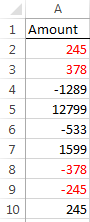
Now, you can’t (easily) sort the numbers because you want to match the negative numbers with the positive numbers so they cancel each other out.
The other challenge is you can’t simply match every instance of a number e.g. 245 is in the list 3 times, twice as a debit and once as a credit.
Excel Bank Reconciliation Formula
Here are a couple of Excel formulas we can use to get our reconciliation done before lunch.
Step 1: In column B create a unique record for every pair (i.e. a pair being a debit and a credit that add up to zero).
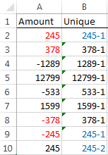
See how the first pair of 245’s are given the value of 245-1, and the 245 in row 10 is given 245-2.
In cell B2 we use this formula:
=IF(A2<0,-A2&"-"&COUNTIF(A$2:A2,A2),A2&"-"&COUNTIF(A$2:A2,A2))
And then copy it down the column.
In English it reads:
If A2 is less than zero i.e. a credit, convert it to a positive number, join a dash to it, then count the instances of the value in A2 in the list A2:A2 and add this number on the end, otherwise take the value in A2, join a dash to it, then count the instances of the value in A2 in the list A2:A2 and add this number on the end.
When you copy the formula down the column the range being counted grows (thanks to absolute references) to include the next row.
Step 2: Identify the pairs in the list.
Now we have a unique list in column B we can identify which values are the same and put a mark against the matches:
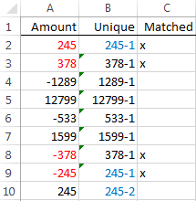
To do this we used this formula:
=IF(COUNTIF($B$2:$B$10,B2)=2,"x","")
In English says:
If the count of the value in B2 in the list B2:B10 = 2, put an x, otherwise put nothing.
Now you can sort the data based on column C and anything without an ‘x’ is not reconciled.
Off to an early lunch. Your work is done 🙂
Enter your email address below to download the sample workbook.
Download the Excel workbook. Note: This is a .xlsx file, please ensure your browser doesn't change the file extension on download.
Thanks
Thanks to Dominique for asking this question. I enjoyed reminiscing about my accounting days.
If you found this useful please share it with your friends and colleagues using the Google+1, LinkedIn, Facebook and Twitter buttons.
If they do any kind of reconciliations they’ll love you for this tip!

Thank you so much. You are a life saver.
Glad we could help!
Awesome, thanks for this!
Our pleasure!
Hi, the formula was helpful. than you
One concern is if the debit and credit amount is same example 1000 debit and 1000 credit, the formula concerts to same sings and matches.
So is there any alternative solution
Hi Srinivas, I’m not sure what the issue is as that’s the idea of the formula. Perhaps you can post your question on our Excel forum where you can share a sample Excel file with your data and desired result. From there we can help you further. Mynda
Hi,
This post was so helpful.
My approach is to search internet and find best solution for bank reconciliation. I will use this formula in my reconciliation sheet.
I also find another website which I got some ideas for bank reconciliation.
https://armarecon.com/user-manual/
hope to help others for their bank reconciliation.
I relay appreciate you for your valuable post.
Hi I am Luis, your approach help in the sense that it speeds up to find the amounts missing on the Bank Statement side and on the CheckBook side also.. Thank you so much..
Glad I could help, Luis 🙂
how can I use Excel to reconcile my ledger bank account by matching it with the bank statement for the same period?
Hi Mohamed,
Without seeing your files, the only answer I can give is already in this article you just read above.
You can try to upload on our forum sample files with your source data, so we can see how it looks, we will try to help.
ACCOUNT NUMBER Add Amount Deduct Amount Total
24 8 0
24 40 0
24 0 3.25
24 0 2
24 0 1.5
24 0 2
24 0 1.5
34 0 5
77 8 0
106 10 0
120 30 0
120 0 1.5
144 1 0
144 20 0
144 1 0
144 1 0
144 1 0
144 1 0
144 0 1.5
144 0 1.5
165 10 0
165 0 4
165 0 1.25
165 0 5
Sir how we will calculate the total front of every entry
if unique id comes again and again with different credit and debit
Please help me for this.
With Regards
Sumit
Is it just an aggregation you need, like this?
ACCOUNT Add Deduct
24 48 10.25
34 0 5
77 8 0
106 10 0
120 30 1.5
144 25 3
165 10 10.25
You can use simple formulas:
=SUMIF([ACCOUNT],[@ACCOUNT],[Add Amount])
Does anyone know if something similar can be done if you are using Power Query?
Hi Bill,
You’d need to number the records first, then split them into two tables of records; one for those numbered 1 and one for those numbered 2. Then compare the two lists with Power Query.
If you get stuck, please post your question on our Excel Forum.
Mynda
I have applied the above formula in my sheet but this formula fails to knockoff the transactions because of multiple currency used. Example One Cr 40k-1 PLD and one Cr 40k-2 EUR, however I have one Dr value 40k in EUR but it didnt show as matched due to currency issue. Please help.
Hi,
You will have to use our forum to upload a sample file, hard to imagine your data. (create a new topic after sign-in)
How can I reconcile using excel to match of the debits and credits , but here I am talking about 7000 lines , and I need to identify the debit and credit for same customer , this is first situation.
Secondly I need to identify the debit and credit with using the B/L number.
Can you please assist me .
Please see below sample.
Customer No Customer Name B/L No Invoice No Amount
1 Rock Enterprize 12345678 123 45
2 Sand Enterprize 32145 321 -45
3 Beast 12345678 258 -45
4 Rock Enterprize 12345678 741 -45
Hi Shiva,
You need to use a formula similar to this VLOOKUP and Match Multiple Criteria. If you get stuck, please post your question on our Excel Forum where you can upload a sample Excel file and we can help you further.
Mynda
My requirement is same as given by Frederik. I want to know if there is formula to match one debit with multiple credits.
Hi Nethra,
The answer is the same as the one Catalin gave to Frederick.
Mynda
Thank you very much.
However, what to do if a credit transaction is a sum sum of more than one debit transactions?
Like this for example:
500
200
300
-1000
Hi Frederik,
Without a unique identifier that ties the credit transactions to that specific debit transactions, it’s almost impossible, you have to dig through all transactions, combine the credit values until one debit transaction matches. And that is most likely a source of errors. Of course, depends on your data and how the information is structured.
Catalin
Hello!
This formula has been extremely helpful. However, I am wondering if I can add a condition to the formula. I need to match debits and credits which this formula helps to do, but the amounts that match off need to be associated with the same contract number. So the condition in my situation would be a contract number.
Any help would be appreciated!
Hi Amber,
Can you upload a sample data sheet so we can see your data structure? Use our forum to upload the file (create a new topic)
Without seeing your data, it’s hard to imagine a solution, thank you for understanding.
Catalin
Hello,
I uploaded a very simplified version of my data in the forum under General Excel Questions and Answers titled “Excel Bank Reconciliation Formula- with condition.”
Thanks!
Hi Amber,
Looks like you already have a solution on forum 🙂
Regards,
Catalin
I have to look the matches in two different columns. How can I do the same thing? Thank you in advance.
Hi,
Can you provide a sample file? You can upload it to our forum: excel-forum (Create a new topic after signing-up)
Catalin
Hi there, would you help me to learn or where to learn about transactions reconciliation between two big transactions. I have an interview coming up on this and am struggling to find enough information. Its nothing specifically in youtube either. Please help. Will really appreciate it.
Hi Mohammad,
Learning how to reconcile accounts is an accounting topic, as opposed to it being strictly Excel related. I’d do some Google searches on ‘how to reconcile accounts’ or similar.
Mynda
I want check bank reconciliation statement please provide formula in excel sheet
Hi Ashok,
There is a downloadable file in this article (here is the link again), so I don’t understand what you mean, please be more specific.
Nice work
Dear
I follow your tutorial articles which are very helpful for me
I applied this formula to my bank reconciliation and it wirked perfectly
A wonderful performance saving a lot of time
Regards
Glad I could help, Hassab 🙂
Thank you so much for sharing. I do run into a problem while using the formular. Sometimes, it could not match a pair of numbers. I can see both the same number like two 100-1 with no match mark made. Do you have any suggestions about where to fix? thank you so much
Hi Jay,
You can open a new ticket on our support system. Make sure you upload a sample file, so we can see a sample of your data, and the error.
Regards,
Catalin
Thank you very much, I’ve been using this tip for some time now, and it has been very helpful. One additional question, if I want to perform this on a monthly batch of transactions but I want to evaluate each day/date independently, how could I modify the formula? I do have a separate date field, but am not sure how to look at the each date separately.
Thanks again for any help you can provide!
Dave
Hi Dave,
Can you upload a sample file? It will be easier for us to help. You can use our forum, just open a new topic: https://www.myonlinetraininghub.com/excel-forum
Catalin
i just want to reconcile the bank reconciliation statement with organizational cash book…i feel it is very difficult task to reconcile easily and quickly,so plz help me for the completion of my assignment.kindly email me your fruitful material and excel sheet for this..
Hi Muhammad,
I’m sorry but I don’t have any template for this. The best I can offer is the formula above. Hopefully you can adapt it to your needs.
Mynda
I just wanted to let you know that your post is still helping people! I have been trying to build my own Auto Reconciliation Excel Add in and this formula finally helped me map out the most challenging part. I did modify your formula a bit so I can import two different sheets and have it match by the category type as well (Checks,Deposits,Expenses)
Instead of having just the -1 added to the end I also add a letter to coincide with the category. In my example K3:K5 hold the values that [@Type] is matched against.
=IF(G4<0,-G4&"-"&COUNTIF(G$4:G4,G4),G4&"-"&COUNTIF(G$4:G4,G4))&IFS([@Type]=$K$3,"C",[@Type]=$K$4,("D"),[@Type]=$K$5,("E"))
After applying the formula to both tables independently, I used a lookup to match the rows between the two tables as well as provide me an bright red warning on unmatched transactions.
Would you have any suggestions for simplifying the formula so it will be more VBA friendly?
Thanks again
Matthew Fulton
Parkway Business Solutions
https://parkway.business
Instead of the last part ( IFS([@Type]=$K$3,”C”,[@Type]=$K$4,(“D”),[@Type]=$K$5,(“E”)) ), you can use a lookup table:
INDEX(Table4[Column2],MATCH([@Type],Table4[Column1],0)), where column1 has those K3, K4 and K5 values, and column 2 will hold the corresponding values: C, D and E.
It’s easier to use table names in vba than to recreate those cells references.
Cheers,
Catalin
Wonderful. best formula for a reconciliation. Thanks
Cheers, Rahul. Glad we could help.
Mynda
excellent formula. Thanks for sharing this and explaining in plain english for the best understanding.
I have copied your formula and pasted it in the excel sheet and did small changes. It works fine. Fantastic.
Thanks 🙂 Glad that we were able to help you out.
Regards,
Phil
Need an help in reconciliation
Hi Vinod,
Do you have a specific question we can help with?
Mynda
Thank you so much! I have been looking for a solution to this for hours. This is the best one by far! Thank you, this has saved me a ton of time! Amanda
Glad it was helpful, Amanda 🙂
Hi, Thank you for this!
But what if you have debits and credits in two seperate columns?
Hi Curston,
Move them into one column 🙂
That’s the easiest solution.
Kind regards,
Mynda
Hi Mynda,
Thanks for sharing. It really helps.
I have a similar situation but rather than only values “amount” in column A, I have one more column , eg column C which includes another query ,eg.”date” or ” payment number”. Is there any way still applying this formula with restraint to column c eg “restriced to particular date or payment number?
Hi Danny,
The key to this technique is to create a unique value from the amount column. We do this by counting the instances of the same number and then apending a 1 or 2 etc. to the end.
But in your case you don’t need to append the 1 or 2 etc. as you can create a unique value by concatenating the amount in column A with the Payment Number in column C (I presume there won’t be more than one instance of the payment number i.e. it is unique to one Debit and one Credit entry only). e.g.:
Note: You don’t have to put hyphen in between each value in column A and C, but it might just make it easier to read if you do.
Once you have your unique value using the formula above, you can apply the matching formula in the same way as the example above.
I hope that helps.
Kind regards,
Mynda.
Hello Mynda,
Please I have a very similar situation to Victor’s but the difference is that the reference number and amount a times appears more than once. After concatenating both the reference numbers and amounts and applying the matching formula above, only one debit and credit were matched. How do I adjust the formula to match both debits and credits as many times as they appear.
I must commend your style of teaching.
Thank you.
Hi Dido,
Can you please upload a sample file with detailed description of what you are trying to achieve? It will be easier to work on your specific structure.
You can use our Help Desk.
Cheers,
Catalin
=IF(COUNTIF($B$2:$B$10,B2)=2,”x”,””)
I will like to amend the matching formula above such that if the count of value in B2 in the list B2:B10 is an even number put an X, if an odd number (say 2 debits and one credit) put an X for every pair of debit and credit and put nothing for the outstanding debit.
Thank you.
Hi Dido,
try this version:
=IF(MOD(COUNTIF(B:B,B2),2)=0,”x”,””)
MOD function will return true id the result of COUNTIF function divided by 2 has no remainder ( the result is an even number).
Cheers,
Catalin
Hi Mynda, i like your way of teaching so much, it shows how much exp u have in this field with real stuff! am using excel more than 5+ yrs but still i can’t learned anything effectively…after saw your real stuff … i like n love to learn more about..it! pls suggest me how can i ask my queries if any? give me your mail id so that it will very useful for me…
Hi Emmanuel,
Thanks for your kind words 🙂
You can learn more from me via my courses:
Advanced Excel Course – Excel Expert
Excel Dashboard Course.
You can send me questions via the help desk.
Kind regards,
Mynda.
hi, thanks a lot for your quick response! kindly update me about your new courses, materials etc., if you have any free material about report generation through macros kindly share with me please! if possible pls send me to my mail id.
Will do, Emmanuel. I’ve added you to our Excel newsletter email list so you will receive our free email tutorials and notices of any new courses or promotions we’re offering.
Kind regards,
Mynda.
Mynda, I have a doubt in preparing the “Reports in excel by using macros” …kindly help me to learn detailed or else send me some sample files or videos?
Hi Emmanuel,
Unfortunately I don’t have any examples I can point you towards. We do have a VBA course in production but it’s not available yet.
I’m sorry I’m not more help.
Kind regards,
Mynda.
Its ok….somehow hard for me…because i have waited for so long years to learn…i hope u will surely help me to learn once its ready or will update me as soon as possible.
Will do, Emmanuel 🙂
I would like to reconcile but with one credit matching multiple debits. Can anyone help with a formula? See below at my example. Thanks Richard
100 x
-25 x
66 xx
-2 xx
-50 x
-4 xx
-60 xx
-20 x
-5 x
Hi Richard,
You could try Solver for this
Kind regards,
Mynda.
Hi Mynda,
You are Superb..
Thanks for sharing your knowledge.
I use Bank Reconciliation formula regularly in my office & it is very helpful.
But I face one problem when I apply this formula after filter. Would you help me out how can I apply this formula after filter where it reads only visible figures..
Waiting for your reply.
Thanks & Regards
Kuldeep Kumar
Hi Kuldeep,
Instead of the =IF(COUNTIF($B$2:$B$10,B2)=2,”x”,””) formula you can use this:
Kind regards,
Mynda.
Hi Mynda,
Thanks for reply to me…(-_-)
Please consider my below problem which is related to bank reconciliation:
There are three funds & every fund has five hundred (500) transactions & all transactions are mixed according to date (some are related to 1st fund & some are related to 2nd fund & so on), which I have to reconcile seperatly by using filter, By FILTER all transactions show into relevant fund because all transactions has a Fund’s head. When I use this formula: =IF(A2<0,-A2&"-"&COUNTIF(A$2:A2,A2),A2&"-"&COUNTIF(A$2:A2,A2))..this formula also reads that figures amount that is same in other funds & also hidden by filter and puts the result like 245-1, 245-2, 245-3 & 245-4….(whether it is to be in negative or positive) in increasing order by reading hidden amount also.
I want that formula, which read only that amount which fund has filtered & visible & not related to other fund. Please explain this new formula in English by using colors.
Waiting for your reply.
Thanks & Regards
Kuldeep Kumar
Hi Kuldeep,
If you use formulas that only pick up the unfiltered data then as soon as you remove the filters the formulas will pick up all data. This means that you can never look at all of the data in an unfiltered state at the same time, and if you inadvertently do, the formulas will give erroneous results.
Would it not be better to sort the data by fund and then separate it into a worksheet for each fund, or at least separate the data for each fund with a few blank rows?
This way the formulas already available above will work and you can get an overview of all funds at the same time. Plus you won’t run the risk of looking at unfiltered data and getting the wrong matched information.
Kind regards,
Mynda.
Hi Mynda,
Thanks for your help.
Would you please explain this formula In English by using colors with a short example of Bank reconciliation in Excel worksheet ( as you have explained Bank Reconciliation formula):
=IF(SUMPRODUCT(SUBTOTAL(3,OFFSET(B2,ROW($B$2:$B$10)-ROW(B2),0)),–($B$2:$B$10=B2))>1,”x”,””)
Thanks & Regards
Kuldeep
Hi Kuldeep,
It’s not easy for me to put colours into the comment fields. I recommend you watch this video on deciphering formulas. You can also read up on the functions used:
IF
SUMPRODUCT
OFFSET
And the ROW function returns the row number for the cell referenced. When used in an array formula like SUMPRODUCT it retuns an array of row numbers. So ROW(B2:B10) with return this array of numbers {2;3;4;5;6;7;8;9;10}.
I hope that’s enough to get you started.
Kind regards,
Mynda.
Hello, I am Luis, regarding Kuldepp Consult of transactions of different funds, I solved this situation by creating a Shortcut (numeric) nickname for each fund.. then I linked this numeric shortcut in a table which I used for the Bank Recon.. This way I could filter each fund transaction and determine which was Paid or Deposited in the month when Reconciling..And as Mynda, suggested at the End of the Recon, you must make an Individual report for each Fund to show the details for each one, Best Regards,
You could make transaction matching easier using Excel add-in – SumMatch.
You may finish your reconciliation before your morning coffee break!
Thanks for sharing, Catpol.
Hi Mynda, just a quick question:
Is there an option to subscribe (via email) to the comments of a particular post on this blog ?
Hi KV,
The comments for any post can be received using RSS. The address for the RSS feed for any post is the post’s URL /feed
So for this post it’s http://www.myonlinetraininghub.com/excel-bank-reconciliation-formula/feed
You can receive the RSS feed using Outlook or an RSS reader like Feedly
Some browsers will recognise the RSS feeds and allow you to subscribe by clicking on the RSS icon in or around the URL bar too.
Regards
Phil
The formula in column C works only on the first and second instance of a value in column A to cancel each other out.
This means if there is a third and a fourth instance (or more), those values will not be flagged with an ‘x’.
Also, I may be wrong about this, but if we check for ABS values of the value in column A, this formula could possibly also cancel out two positive entries or two negative entries.
We may need to add one more column with a formula to ensure that only a positive and a negative number are cancelling each other out.
One other thing: if the data is sorted by column C, wouldn’t the formulas in that column be affected due to the relative references in columns B and C ?
It may be a good idea to convert the formulas in column B and C to values before sorting the table.
Or better still, just filter column C on records with an ‘x’.
Hi KV,
Thanks for your comments.
The formula in column B does two things:
1. It creates a unique value by appending the -1 or -2 etc. to each value. This is for the purpose of matching in column C.
2. It decides what the appended value is by by counting how many of the same values there are in the list. So if there are 3 positive 245 amounts each one will be numbered 245-1, 245-2, 245-3 and if there are only two negative 245 amounts they will be given the value of 245-1, 245-2. So although you have two 245-1 values in column B, one represents the positive and one represents the negative.
This way you won’t have a case where two positive values contra each other out, plus it handles multiple instances of the same values cancelling each other out by giving each pair (postive and negative) a new unique value in column B e.g. 245-1, 245-2.
Perhaps if you download the workbook you can test some scenarios and see how the formulas work.
In regards to pasting as values before sorting, yes you are correct, you need to do this. Or like you say, simply use filters.
Kind regards,
Mynda.
P.S. You should receive an email when new comments are posted to this blog entry.
Thanks for the clarifications Mynda 🙂
I *was* wrong after all, about the way the formula in column B works
And I haven’t received any email so far (checked my SPAM folder too).
Unless, it works only when a “new comment” is posted, and not replies to older ones ?
Nice Excel blog
You could simplify your first formula by using the ABS function
=ABS(A2)&”-“&COUNTIF(A$2:A2,A2)
The ABS function (short for Absolute) converts all negatives to positives.
Cheers, Neale. Great tip 🙂
Hi Mynda,
Thanks for sharing this trick.
It would be great if you can share one spreadsheet with one complete illustration on this topics.
Waiting for your early reply.
Thanks and Regards
CA Sonu
Hi Sonu,
You’re welcome. You can download the Excel workbook here. Note: this is a .xlsx file, please ensure your browser doesn’t change the file extension on download.
Kind regards,
Mynda.