Numbering items within grouped data is easy with an Excel COUNTIF formula, but numbering grouped data in Power Query requires a few more steps. For example, taking the data below, in column C I’ve numbered the Sub Areas within each Area:
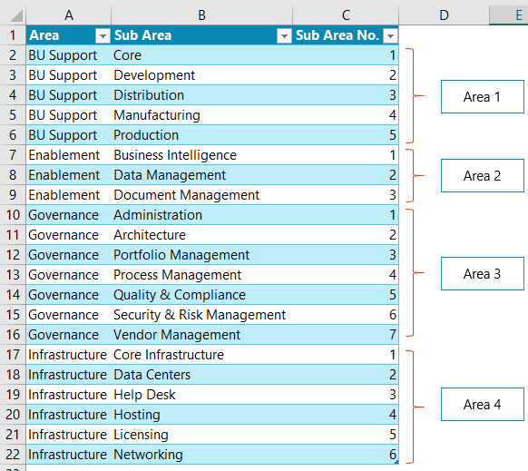
Notice they don’t all have the same number of sub areas.
Download the Workbook
Enter your email address below to download the sample workbook.
Steps for Numbering Grouped Data in Power Query
Step 1:
I started by formatting my source data in an Excel Table, called ‘Table1’: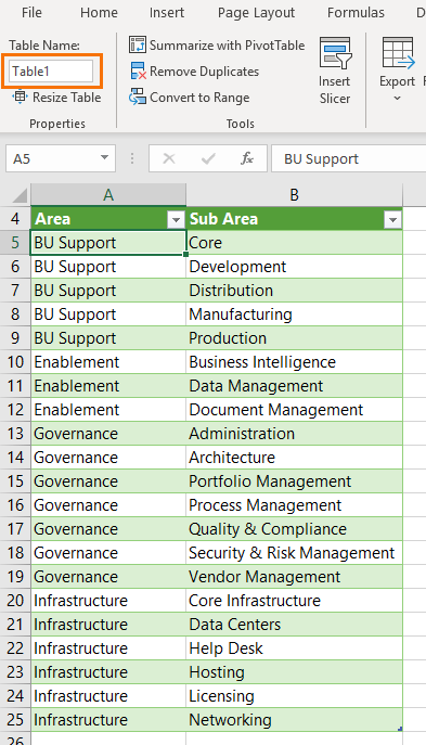
Step 2:
Load to Power Query. In Excel 2016 onward go to the Data tab > From Table/Range: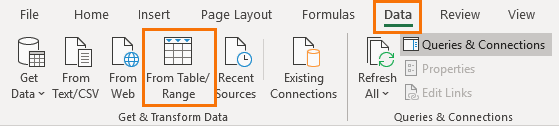
In earlier versions of Excel go to the Power Query tab > From Table.
This will load the data to Power Query and launch the Power Query Editor window.
Step 3:
In the Power Query editor window Add an Index Column (Note: this step isn't strictly required in this scenario, I just added it out of habit)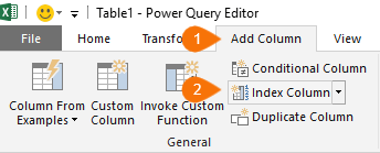
Tip: the index can start at 0 or 1 as it makes no difference.
Step 4:
Group Rows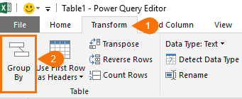
This will open the Group By dialog box:
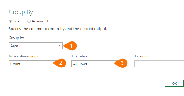
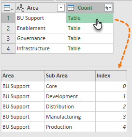
The data is now grouped into tables for each Area. Clicking in the white space beside one of the ‘Count’ column’s tables displays the underlying data in the preview pane at the bottom of the Power Query window, as you can see below:
Step 5:
Add a Custom Column to index each grouped table: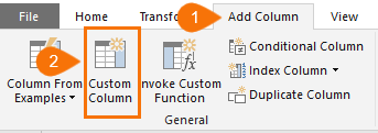
Use the Power Query Table.AddIndexColumn function to Index the Count column created in the previous Group By step:
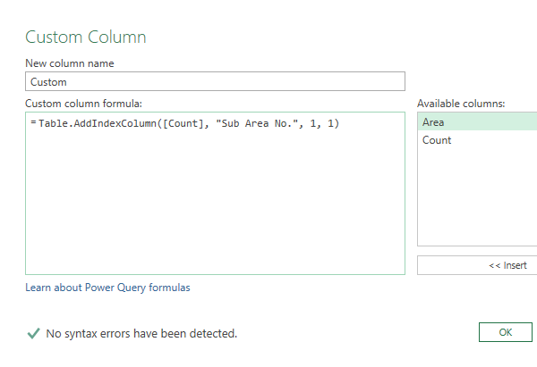
In English the formula translates to:
= Table.AddIndexColumn([Count]. Call this new column "Sub Area No.", 1, 1)
Add an Index column to the individual tables in the [Count] column called ‘Sub Area No.’. starting the numbering at 1 and increment by 1
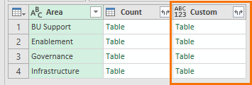
In the Power Query editor window, we now have a new column called ‘Custom’ that contains our individually indexed tables we just added:
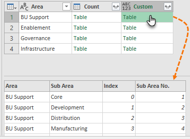
If you click in the white space beside one of the Tables in the ‘Custom’ column you’ll see a preview showing the new column for Sub Area No.:
Step 6:
Delete the Count column as we no longer need it. Just select the Count column header and press the Delete key: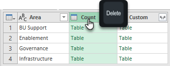
Step 7:
Expand the Tables in the Custom column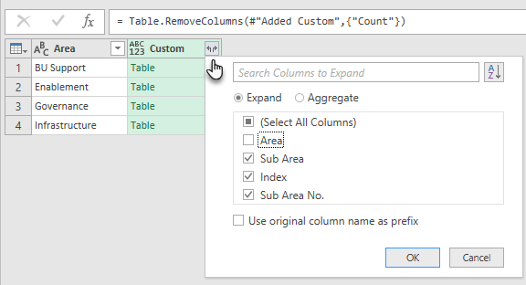
Notice that I deselected the ‘Area’ column as we already have this. And I’ve deselected ‘Use original column name as prefix’.
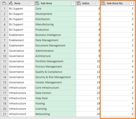
Now I have my tables expanded and the ‘Sub Area No.’ column contains index for each Area:
Step 8:
Delete the ‘Index’ column as we no longer need it.Step 9:
Set the Data types for each column by clicking on the data type icon in the left of each column header: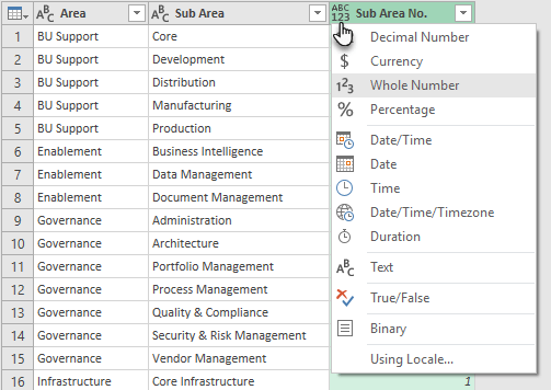
Step 10:
Close & Load. Now you’re ready to close the query editor and load it to a Table in the Excel workbook, or the Data Model a.k.a. Power Pivot, or a PivotTable etc.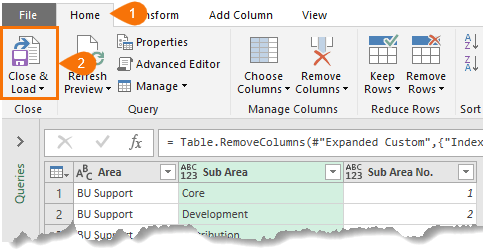
Numbering Grouped Data in Excel
If you don’t need your data numbered in Power Query you can achieve the same results with an Excel COUNTIF formula like so:
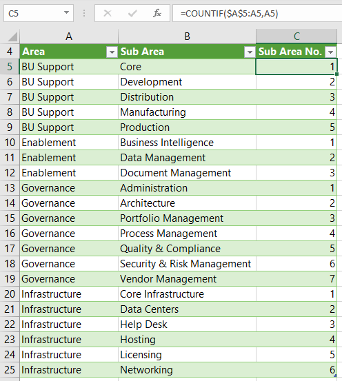
Pay close attention to the use of absolute and relative references:
=COUNTIF($A$5:A5,A5)
Thanks
Thanks to fellow Excel MVP, Ken Puls, for pioneering the Power Query technique here.
Please Share
If you liked this please share it with your friends and colleagues.


This is excellent material! I saw this method elsewhere at one point, but when I went looking for it again, I came across this and this is much better presented. Thanks!
Thank you Joe for your feedback!
Agreed! Thanks for the easy step-by-step!
This came in super helpful. Thanks for taking the time to write and post this!
Our pleasure, David 🙂
Amazing capability and well-written instructions. Thank you for sharing!
Thanks so much, Dror! Great to know it was helpful.
So I did this for a field in my table called Locations. (I’m trying to count the number of open tickets for each corporate location and my main table contains ALL open tickets). How would I finish this off by doing that – example
albany – 7
Allentown – 6
ect.
Thanks in advance if you have time to answer. I appreciate it.
Hi Randall, I’d use a PivotTable to do the count by location. If you’re stuck, please post your question on our Excel forum and you can upload a sample Excel file so we can help you further.
This saved my bacon. Thank you!
🙂 glad I could help!
Thanks for this, very straight forward and simple to follow
Glad you found it helpful, Yolandi!
You’re welcome
Hello,
Much appreciate the step by step process. Just what I needed! To go one step further I had to find the maximum value within the “Subarea” column to thus do a filter. Table.max to the rescue! Could not have done it without you. Thanks indeed!
Glad I could help, Sylvain! 🙂
Thank you very much for this super-useful post. I often need to use such a grouping in my data. However, I had an issue where, after expanding the Custom column, data types I had previously set or modified went lost and each column in the table had reverted to data type: Any. Can you help shed some light on this issue?
Hi Francesca,
This is common in Power Query, i.e. many processes will remove the data type settings. I recommend using the ‘Detect Data Type’ tool on the Transform tab to quickly set data types again.
Mynda
Important note: If your list is sorted, the sorting and indexing may be unstable or incorrect. To avoid this issue, you can surround your Table.Group code with the Table.Buffer function in the advanced editor, so that the sort order remains stable.
Here is an example that buffers, groups and adds the index all in one line:
#”Grouped Rows” = Table.Buffer(Table.Group(#”Sorted Rows”, {“SpecialityID”, “DesignationID”}, {{“GroupedRows”, each Table.AddIndexColumn(_,”Index”,1,1), type table}})),
Here are some references to this issue:
https://www.excelando.co.il/en/powerquery-remove-duplicates-bug-workaround/
https://social.technet.microsoft.com/Forums/WINDOWS/en-US/30e9ab27-23a5-465b-a0c4-36e4e48ce2db/bug-or-feature-when-querying-sqlserver-data?forum=powerquery
Thanks for sharing, Neil.
You literally saved my life. I was doing this with a table that was transactions per product ID. I wanted to have the last transaction per product and per date ( for each transaction). When I did the self join, everything got messed up. Thank you very much.
Glad I could help 🙂
Hi – I downloaded the Excel workbook from the shortcut in the post and Windows 10 professional reported a Trojan virus in the file: Win32/Spursint.F!cl
Hi Frans,
This is an issue with your Windows Defender software. If you search for ‘win32/spursint.f cl false positive’ you’ll see many mentions of this issue.
If you want to be sure, you can go to https://www.virustotal.com/#/home/url and supply the URL to the workbook and VirusTotal will scan it for you.
I’m happy to email the file to you if you like?
Regards
Phil
Thanks Phil for the quick reply and my apologies for raising this when it has turned out to be a ‘false positive’ – I thought it best to report it to you in case it was a real virus. Thanks for the offer to email the file – but I have recreated the sample data manually. PS: I always find your site’s training programmes and newsletters very informative. Kind regards, Frans
Hi Frans,
No worries, always best to be safe.
Great to know you enjoy our site and newsletters.
Thanks
Phil
Mil gracias Mynda, entendi la formula de Table.AddIndexColumn :). muchas gracias por los post siempre son geniales y aprendo mucho. Te envio un fuerte abrazo!.
De nada 🙂
What do we need the first index column for?
Good question, Adrian! In this scenario you can get away without the first Index column, but often you’ll find you need it to avoid getting an Expression Error. I just added it out of habit 🙂