A few weeks ago David T asked me to help him understand a VLOOKUP formula in a workbook he’d inherited from a colleague who had left his company.
It was a VLOOKUP formula like nothing I’d ever seen before so I thought I’d share it with you.
Drum roll…..
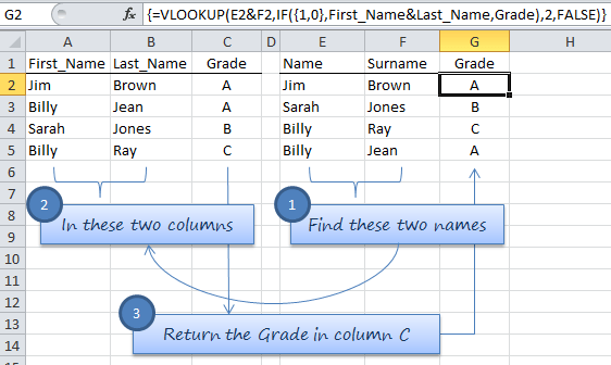
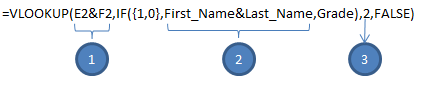
=VLOOKUP(E2&F2,IF({1,0},First_Name&Last_Name,Grade),2,FALSE)
David’s question was ‘what’s the IF({1,0},… doing’?
First here’s the Excel workbook used in this tutorial if you want to download it.
Enter your email address below to download the sample workbook.
Ok, before we dive in and try to understand the IF({1,0} we'll start by remembering the syntax for VLOOKUP:
VLOOKUP(lookup_value, table_array, col_index_num, [range_lookup])
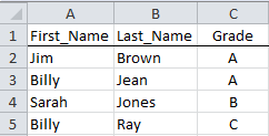
Let’s look at an example (I’ve recreated some dummy data as David didn’t send me his file):
Note: I’ve given the columns A, B and C the following named ranges which are referenced in the formula:
- A2:A5 = First_Name
- B2:B5 = Last_Name
- C2:C5 = Grade
The formula in cell G2 is looking up the names in E2 & F2 and finding matching values in column A (First_Name), & B (Last_Name) and then returning the result in column C:
How Does it Work?
Firstly this is an array formula so it must be entered with CTRL+SHIFT+ENTER.
- The formula uses an ampersand (&) to concatenate/join the lookup_values in E2 & F2 like so:
- The IF function creates a matrix, which is the table_array argument for the VLOOKUP formula which consists of two columns.
- Lastly the col_index_num simply tells Excel to return the value in the second column of the table_array i.e. the Grade.
=VLOOKUP(JimBrown, IF({1,0},First_Name&Last_Name, Grade),2,FALSE)
Remember the syntax for the IF function is:
IF(logical_test,[value_if_true],[value_if_false])
The {1,0} matrix are numerical equivalents of TRUE and FALSE and are the logical_test argument for the IF Function.
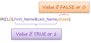
Note how the value_if_true argument also uses the ampersand to join the First_Name’s & Last_Name’s together.
In the formula it evaluates like this:
=VLOOKUP("JimBrown",{"JimBrown","A";"BillyJean","A";"SarahJones","B";"BillyRay","C"},2,FALSE)
Where commas separate columns, and semi-colons separate rows.
You might find it easier to visualise the table_array like this:
Special thanks to Roberto for helping me decipher this formula.
VLOOKUP vs INDEX & MATCH
As I said, I’ve never seen it done this way. I would have used INDEX & MATCH.
Remember VLOOKUP’s sibling is INDEX & MATCH. Some might say INDEX & MATCH is the better looking/more elegant sibling. What VLOOKUP can do, INDEX & MATCH can usually do better.
Here’s how:
=INDEX(Grade,(MATCH(E2&F2,First_Name&Last_Name,0)))
Also entered as an array formula with CTRL+SHIFT+ENTER.
What Do You Think?
Whilst I enjoyed learning this VLOOKUP & IF function trick I still prefer INDEX & MATCH for this type of challenge. It’s not only a shorter and more efficient formula than VLOOKUP & IF, I think it’s also easier to understand.
Have you seen this before? What do you prefer; VLOOKUP & IF or INDEX & MATCH? Let me know in the comments below.

I want a formula for same item with different price in different rows and select the any price required when selected from data validation. I have data validation in another sheet but it takes value for the first row price in another sheet.
Hi Vipul,
Please post your question on our Excel forum where you can also upload a sample file and we can help you further.
Mynda
Hello! I am trying to use a lookup for my ordering sheet but I am trying to find the logic to formulate it but I haven’t been able. So I create an excel with 3 sheets. One is the Ordering Form. another one the product list with the name, price, half case and bottles, and the order one with my customers. For example, I sell wine by the case which are 12 bottles in the case, but some wines come in cases of 6 bottles only or maybe the customer wants to buy only 2 bottles of wine. So in my productList I have 1 column with the name of the wine, another one with the cost per case of 12 bottles, next column I have the price for 6 bottles, and the last the price per bottle. How can I formulate this in the Order Form sheet? I need when is a 6 pack takes the price of 6 not a full case
Hi Marjorie
You should use an INDEX-MATCH combination, here is a link to a tutorial that will help.
Your formula should look like this:
=INDEX(tablerange, MATCH(A1, D5:D20, 0), MATCH(B1, C4:F4, 0))
where: A1 is the wine name, B1 should be the number of bottles per case. D5:D20 will be that range where you have the wine names list, C4:F4 is the range that contains the numbers of bottles per case headers.
Thank you so much, Catalin for the information
You’re welcome!
Here is something that may be of use to some when using VLOOKUP to add multiple columns of figures (HLOOKUP if rows of course). When adding a couple of columns I was using:
=SUM(VLOOKUP(A31,HideSheetMains!$A$5:$H$78,4,0),VLOOKUP(A31,HideSheetMains!$A$5:$H$78,8,0))
I had 8 columns I needed to add within a much larger calculation so I stumbled upon this method; the curly brackets are typed in, not ctrl+shift+enter:
=SUMPRODUCT(VLOOKUP(A31,’BMS Sub Calcs’!A5:AO78,{34,35,36,37,38,39,40,41},0))
As you can see the data table had 78 columns with many many calculations needing to be carried out.
Thanks for sharing, Joseph.
It’s excellent but I want it from different sheet. Is it possible ?
Hi Harun,
The names you saw in this tutorial (First_Name,Last_Name,Grade) are workbook level defined names, the data can be in any sheet. Simply set the names to our data ranges and use them in formula.
Catalin
I use VLOOKUP for the optional subject means if there is two subject as optional. A student have to choose one and that mark will add to the result . If Roll Number one take 1st optional and roll no-2 take 2nd optional . I also set a rule for blank . If i press roll no 2 the value shown as i want in look up but the formula result give me blank.
Hi Mrutyunjay,
Please post your questions and a sample Excel file on our Excel forum so we can help you. Your question here is difficult to understand without an example.
Thanks,
Mynda
It is good. But I want to know the formula o v lookup function. I use the V LOOKUP function and result is Blank. It shows a vlue after look up but the formula result show blank.
Would this have been easier by inserting an extra column and concatenating the first and last name? Then using vlookup or index+match?
Hi Harold,
Sure, you could do that for both tables, but often people want a solution that doesn’t require extra manipulation of the data.
Mynda
i want in my excel sheet remarks collom 0= CLEARE, IF NOT 0 = NOT CLEAR
LIKE PENDING AMOUNT 500= NOT CLEAR. 0 =M CLEAR HOW?
Hi Manu,
Try a simple IF formula:
=IF(A1=0,"Clear","Not Clear")If you copy this formula down as needed, you will get the “Clear” result only for cells from A column that are 0 or empty.
Cheers,
Catalin
Another Question: What does CTRL+SHIFT+ENTER do? It is said, that it’d be entered with it b/c it’s an array formula?
Hi Diana,
An array formula requires entering differently to a regular formula. i.e. with CTRL+SHIFT+ENTER. You can read more about array formulas here.
Kind regards,
Mynda.
Mynda,
on #3, “Lastly the col_index_num simply tells Excel to return the value in the second column of the table_array i.e. the Grade.” – did you mean the second or third column?
Diana
Hi Diana,
That’s a great question. I meant the second column and this is because we are using the & to join column A and B together so from Excel’s point of view they are the first column and column C is the second column.
I recomment you use the Evaluate Formula tool to follow the logic and evaluation steps of this formula so you can see how it is working under the hood. Here is a video I recorded on troubleshooting formulas and understanding how they work.
Kind regards,
Mynda.
Dear sir/madam
when i am puting vlookup farmula in worksheet its not working,is it running with vba code ? if yes plese send us also vba code
thanks
jiwan singh
Hi Jiwan,
It doesn’t require VBA but it is an array formula which means you need to enter it by pressing CTRL+SHIFT+ENTER.
You can read more on array formulas here.
Kind regards,
Mynda.
Hi Mynda,
You wrote: Lastly the col_index_num simply tells Excel to return the value in the second column of the table_array i.e. the Grade.
The grade is in column C, so isn’t the third column of the table array?
Thanks in advance for your reaction.
Kind regards, Eric
Hi Eric,
Good observation, but because we are joining the first and last names together inside our formula, they become the first column and the grade becomes the second column.
When you look at the formula as it evaluates we can see the comma separates the data into columns and the semicolon onto a new row:
=VLOOKUP("JimBrown",{"JimBrown","A";"BillyJean","A";"SarahJones","B";"BillyRay","C"},2,FALSE)If we were to view the lookup_array above in a tabular format it would look like this with two columns of data:
JimBrown A
BillyJean A
SarahJones B
BillyRay C
I hope that helps.
Kind regards,
Mynda.
Dear Mynda,
You are Awesome!
thank you for your share ..
louay
Thank you, Louay 🙂
Great little trick with vlookup. I haven’t done much with arrays on my reports but it looks very powerful way of referencing data. I prefer index & match 🙂
Thanks, Edwin 🙂
thank you, it’s great post. i never thinking this way before, i prefer use index and match easier than vlookup & if.
Thanks, Effendi 🙂
Awesome. Good to know about that. I have never seen such construction before 🙂
The similar formula with CHOOSE instead of IF could be:
{=VLOOKUP(E2&F2,CHOOSE({1,2},First_Name&Last_Name,Grade),2,0)}
CHOOSE is more fexible than IF because you can create an array with more than 2 columns 🙂
Recently, I explained one of my students VLOOKUP/CHOOSE and INDEX/MATCH/. She went with INDEX/MATCH because she said it was easier to understand 🙂
Cheers, Pmsocho 🙂 I like your CHOOSE option too.
I wrote a tutorial on VLOOKUP and CHOOSE here, but with just a single lookup value.
Kind regards,
Mynda.