A little while ago Brendan asked me how he could check if values in a list fall between two limits.
Now, it’d be nice if there was a BETWEEN Function, but there isn’t. Hence why the title of this tutorial isn’t ‘BETWEEN Function’, it’s ‘BETWEEN Formula’.
I’ve got two options for you.
Watch the Video

Download Workbook
Enter your email address below to download the sample workbook.
Excel BETWEEN formula using AND
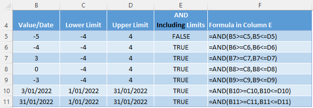
In the example table below I’m checking if the value/date in column B falls within and inclusive of the upper and lower limits:
In English, the formula in cell E5 simply reads: is the value in B5 greater than or equal to the value in cell C5 (the lower limit) AND less than or equal to the value in cell D5 (the upper limit)?
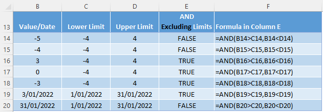
If you strictly want to check if a value/date falls between the upper and lower limits, you can omit the equals sign from the formulas like so:
Excel BETWEEN formula using MEDIAN (Inclusive)
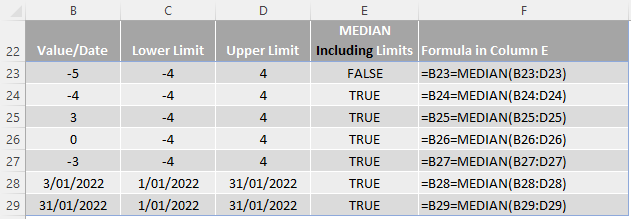
The MEDIAN function returns the middle value in a set of 3 numbers. If the value is between two values, then it will be returned by MEDIAN, which makes it perfect for this task.
Taking the examples above, the formula in English reads: does the value in B23 equal the median of the value, lower limit, and upper limit? It’s inclusive of the upper and lower limits, as we can see by the results on rows 24 and 29.
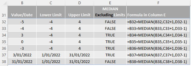
If you prefer to exclude the upper and lower limits, you can add/subtract 1 to the lower and upper limits respectively, as shown below:
Thanks
Thanks to Roberto for the MEDIAN solution.


I have this formula that doesn’t seem to work, appreciate if you can let me know how to go around with it 🙁
=IF(EACP>100,”Red”,IF(EACP>9070<90,"Yellow",IF(EACP<70,"Green"))))
Hi Silahis,
Try this:
=IF(EACP<70,"Green", IF(EACP<90,"Yellow", "Red"))
for EACP of 90 and up will return red. If you want another level:
=IF(EACP<70,"Green", IF(EACP<90,"Yellow", If(EACP<100, "Blue", "Red")))
You should know that nested if's are evaluated until the next logical test is true, the remaining logical tests will not be evaluated.
Your BETWEEN MEDIAN exclusive solution (at least the idea that it’s plus/minus 1 by default) only works with whole numbers. Say you have Value = 4.5, Upper = 5, and Lower = 2. Then using plus/minus 1 as the default ends up with MEDIAN(4.5,2+1,5-1) = MEDIAN(4.5,3,4) = 4 and returns FALSE instead of TRUE. Of course it could work with some other plus/minus shift as long as that shift was appreciably small compared to the size of any possible decimal fractions.
In the end, the MAX MIN approach seems more manageable, particularly if you don’t know which number should serve as the upper/lower limits. Otherwise you would just use direct comparisons as Bryan described. But I don’t really see the point of including a negative sign in the MAX portion, and have to disagree that making it inclusive should be accomplished by increasing/decreasing the limits by 1 as opposed to simply tacking an “or equal to” onto one or both of the inequality signs.
=AND(A3<=MAX(B3,C3),A3>=MIN(B3,C3))
Mynda, it’s “ole Mort” in Dallas, Texas….Hey Happy Mother’s Day to you – let them spoil you today – smile.
I have a Table of data on one worksheet – very simply as an example
3 columns
0 10 -20%
11 20 -10%
21 30 0
31 40 +15%
41 50 +20%
I have a “value” on another worksheet in a Table row, say it is 36, I want to use MEDIAN to find that I should use a factor of +15%.
Am also confused with referencing data in Tables on other worksheets and [@headername]
Most often when I begin typing the reference header name it will appear with others in a list, now it’s not, the names I’m using are LowerValue and UpperValue.
Thanks for any suggestions Mynda…
Mort Wakeland, Dallas, TX
Hi Mort,
I’d use a VLOOKUP on a sorted list to return the factor or +15%. Here is an example:
https://www.myonlinetraininghub.com/excel-2007-%e2%80%93-vlookup-sorted-list-explained
Not sure what’s going on with your table references but have you tried using your mouse to select them instead of typing them in?
Mynda
P.S. had a lovely Mother’s day, thanks!
Hi Morton,
Hope you and Mynda don’t mind if i give you another option to solve your problem, in fact, i think you are already familiar to this solution:
If the data you provided is in range A2:C6 (only data, no headers), then you can use this formula:
=INDEX(C2:C6,MATCH(A10,A2:A6,1)) , where A10 holds the value to be searched (that 36 you mentioned).
The ranges can be hard typed into the formula, like this:
=INDEX({-0.2;-0.1;0;0.15;0.2},MATCH(A10,{0;11;21;31;41},1))
The result is exactly the same, of course.
But if you are looking for an interpolation, to give the precise percentage, even if your data table has a higher granularity, you can try the interpolation formula and a nice interpolation UDF i made as a student.
The sample file can be downloaded from MOTH OneDrive Folder.
Cheers,
Catalin
Your first formula doens’t work if your upper limit and lower limit are both negative numbers, and the value you compare against is positive. For example, if Value = 3, Upper Limit = -2, and Lower Limit = -4, then the formula evaluates to: AND(3MIN(-4,-2) –> AND(3-4) –> AND(TRUE,TRUE) –> TRUE.
Couldn’t you just use =AND(A3C3)?
Hi Bryan,
Thanks for your comment. Another good reason to use the MEDIAN method as opposed to the MAX and MIN option.
I’m not sure what you mean by ‘just use =AND(A3,C3)’, where are you using them?
Kind regards,
Mynda.
Sorry about that, it looks like it treated my greater than and lesser than signs as an HTML tag and removed them (some of my formula explanation is missing as well). The formula was supposed to be =AND(A3 {lesser than} B3,A3 {greater than} C3).