Return the First and Last Values in a Range

• Share on Facebook.
• Share on Twitter.
• Share on Google+
• Share on LinkedIn
• Pin It!

I’ve been asked many times how to find either the cell reference of the first or last value in a range, or even return the values from those cells, and there are many ways to do it.

As usual I'm going to share the methods I think are the best.

Note: the difference between returning the value or cell reference is subtle yet significant. You’ll see later.

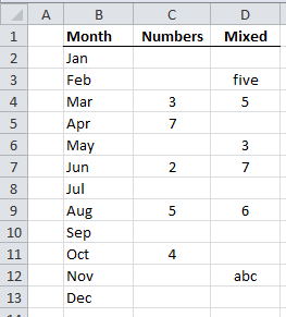
Here’s our range. You can see that column C contains numbers and column D contains both numbers and text, and both columns contain blanks.

Find the First Value in a Range

Like I said, I’ve seen many ways to find the first value in a range but one formula stands out from the rest for its simplicity.

Drum roll…..

=INDEX(C$2:C$13,MATCH(TRUE,C$2:C$13<>"",0))

Entered with CTRL+SHIFT+ENTER as it’s an array formula.

Why it’s so special:

1. The INDEX function returns a reference to a cell and when used on its own, like the above example, it returns the value in that cell.
2. This formula works with text or numbers.
3. The blanks are handled by the logical test in the MATCH part of the formula: C$2:C$13<>""

How it Works

If you’re new to the INDEX & MATCH dynamic duo take a few moments to read this tutorial first. These are two 'must know' power functions.

The MATCH function is the star in this formula:

MATCH(TRUE,C$2:C$13<>"",0)

In English it reads:

Tell me what position (in the range C2:C13) the first TRUE result is in by testing each cell in the range C2:C13 to see if they are not (<>) blank (""), return TRUE for cells that aren’t blank and FALSE for cells that are blank, match it exactly.

If we look at how the MATCH function evaluates it looks like this:

Step 1: Evaluate the logical test and return an array of TRUE and FALSE values:

MATCH(TRUE, {FALSE;FALSE;TRUE;TRUE;FALSE;TRUE;FALSE;TRUE;FALSE;TRUE;FALSE;FALSE},0)

Step 2: Return the position number of the first ‘TRUE’ result in the array:

3

That is the first TRUE is the 3^rd item in the array returned by the logical test.

If we give this result to the INDEX formula we get:

=INDEX(C$2:C$13,3)

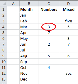
Which evaluates to cell C4 and coincidently the value in C4 is 3.

That is cell C4 is the 3^rd cell in the range C2:C13 and it contains the number 3.

That’s it! Done.

Find the Last Value in a Range

Unfortunately finding the last value in a range isn’t quite as straight forward as finding the first, but it’s not too tricky.

=INDEX(C$2:C$13,MAX(IF(C$2:C$13<>"",ROW($A$1:$A$12))))

Again entered with CTRL+SHIFT+ENTER as it’s an array formula.

Let’s zoom in on the MAX(IF part of the formula:

MAX(IF(C$2:C$13<>"",ROW($A$1:$A$12)))

In English:

Test the cells in the range C2:C13 for blanks, if they’re not blank i.e. TRUE then return the corresponding number from the array of values returned by the ROW function, now just tell me the MAX value.

It evaluates like so:

Step 1 - evaluate the logical test:

MAX(IF({FALSE;TRUE;TRUE;FALSE;TRUE;TRUE;FALSE;TRUE;FALSE;FALSE;TRUE;FALSE},ROW($A$1:$A$12)))

Step 2 - evaluate the ROW function:

MAX(IF{FALSE;FALSE;TRUE;TRUE;FALSE;TRUE;FALSE;TRUE;FALSE;TRUE;FALSE;FALSE},{1;2;3;4;5;6;7;8;9;10;11;12}))

Step 3 - complete the IF formula by replacing the TRUE’s with the corresponding numbers returned by the ROW function:

MAX({FALSE;FALSE;3;4;FALSE;6;FALSE;7;FALSE;10;FALSE;FALSE})

Step 4 – find the MAX of the values:

10

Now we can give that 10 to INDEX and we get this:

=INDEX(C$2:C$13,10)

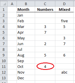
=C11, and the value in C11 is 4.

This formula works for both text and numbers.

Find the Last Number in a Range

If your range contains only numbers, you can use this formula to find the last cell containing a number in the range:

=INDEX(C$2:C$13,MATCH(1E+100,C$2:C$13,1))

Note: for a change this isn’t an array formula.

The trick with this formula is the 1E+100.

1E+100 is just a really big number. You can use any number here as long as it is bigger than any number in your range.

Side note: You might have seen 9.99999999999999E+307 used in formulas before and that's because it's the biggest number you can enter into Excel.

The problem with 9.999 blah, blah, blah is that I find it really hard to remember how many 9's to enter. Whilst 1E+100 is not the biggest number, it is still big enough to work in most scenarios and comes with the bonus that it's a whole load easier to remember.

Ok, sorry I digress... when you ask MATCH  to find a number that is bigger than any of the numbers in your range it will return the position of the last value in the range when you use 1 (for less than) as the 'match_type' argument.

Remember the syntax for MATCH is

MATCH(lookup_value, lookup_array, [match_type])

So in English MATCH(1E+100,C$2:C$13,1) reads:

Lookup the biggest number you can imagine, in the range C2:C13, if you can't find it then return the position of the last number you find.

Remember this formula only works with numbers, not text.

Using INDEX to Return a Reference

So, what about that comment I made in the beginning:

“The difference between returning the value from a cell or a reference to a cell is subtle yet significant”

Well, since we know that the INDEX function returns a reference to a cell we can use the above formulas to return a range that starts with the first occupied cell and ends with the last.

To do this we simply join the two formulas together with a colon, which is the range operator:

INDEX(C$2:C$13,MATCH(TRUE,C$2:C$13<>"",0)):INDEX(C$2:C$13, MATCH(1E+100,C$2:C$13,1))

Remember the first INDEX formula returns a reference of C4 and the second returns C11 so the above formula returns the following range:

C4:C11

What’s the point when you could just enter C4:C11? Well, because using INDEX gives us a dynamic range that will grow or shrink with your data.

Don’t forget if your range contains text you need to use the MAX(IF version:

=INDEX(C$2:C$13,MATCH(TRUE,C$2:C$13<>"",0)):INDEX(C$2:C$13,MAX(IF(C$2:C$13<>"", ROW($A$1:$A$12))))

In most cases you’ll need to enter a formula containing either of the above dynamic ranges using CTRL+SHIFT+ENTER, or you can set it up as a dynamic named range for use in your formulas.

Share This

If you liked this or know someone who could use it please click the buttons below to share it with your friends on LinkedIn, Google+, Facebook and Twitter.