I stumbled upon an interesting question the other day, which was; ‘how do I find the average of a range of numbers that meet criteria, and by the way, I want to exclude the outliers?’
Now, if all we needed was a simple average that met criteria we could use an AVERAGEIF or AVERAGEIFS formula.
Or if we just wanted to exclude the outliers we could use the TRIMMEAN function which returns the mean (average) of the interior proportion of values.
The syntax is:
TRIMMEAN(array, percent)
Where the array is the range containing your values and percent is the fractional number of data points you want to exclude from the top and bottom of your data set.
But we want to effectively find the AVERAGEIF and TRIMMEAN.
Unfortunately this pair don’t get on so well in the same cell so I’ve got an alternative and it’s not called TRIMMEANIF….but maybe there’s an idea.
Note to self; write to Microsoft suggesting new TRIMMEANIF function!
Ok, let’s take this list as our example:
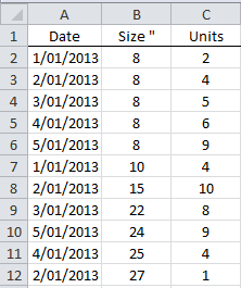
And let’s say we want to find the average Units for Size 8 and exclude the top and bottom 40%.
Note: you wouldn’t normally exclude 40% of your sample but since mine is so small (so it’ll easily fit on the screen) I have had to make the proportion to exclude quite large.
Here’s the formula:
=TRIMMEAN(IF(B2:B12=8,C2:C12),40%)
It’s an array formula so you need to enter it with CTRL+SHIFT+ENTER.
In English it reads: Find the MEAN (average) of the values in the range C2:C12, where the size in the range B2:B12 is 8, oh, and by the way, ignore the top and bottom 40% of the values.
My nested IF formula returns an array of Units that are size 8, and if we step through how the formula evaluates we can see it looks like this:
Step 1: Evaluate the IF formula logical test and expand the range C2:C12
=TRIMMEAN(IF({TRUE;TRUE;TRUE;TRUE;TRUE;FALSE;FALSE;FALSE;FALSE;FALSE;FALSE}, {2;4;5;6;9;4;10;8;9;4;1}), 40%)
Step 2: create an array of the values that evaluate to TRUE
=TRIMMEAN({2;4;5;6;9}, 40%)
Step 3: strip out the outliers from the array of values
=TRIMMEAN({4;5;6})
Step 4: find the mean (average) of the remaining values
=5
Note: if you run this formula through the Evaluate Formula tool you will see it work through the steps above.
Average Top 3 Values
Another member of the Average family that you might find useful is the AVERAGE LARGE formula which finds the average of the top 3 values.

Hi Guys,
It works for me, does what it is supposed to, however, is there any way to make it faster by replacing the IF part somehow?
I mean, I have a huge data on 2-3 different tabs and I need to calculate trimmed mean along with percentile 2 times for min and max and it is very slow to update anything. Is the IF part replaceable by alternative like INDEX/MATCH? Would it be faster? Any Idea? Thanks.
Hi Istvan,
It’s difficult to offer an alternative without seeing your scenario and criteria for the mean. It might be that you can use PivotTables, or maybe Power Query to extract the data excluding the outliers. Please post your question on our Excel forum and include a sample Excel file. From here we can help you better.
Mynda
Alternative, ommiting top 5%:
=AVERAGE(INDIRECT(“BH”&COUNTA(BH:BH)-ROUNDDOWN(COUNTA(BH:BH)*0.95,0)&”:BH”&COUNTA(BH:BH)))
Assuming BH is where you have your data range, and that your data range is sorted descending.
🙂
If you sort it ascending, you get the bottom 5% ignored. 🙂
Perfect! Thank you. It was exactly what I needed (although I would have saved myself 20 minutes if I had read the next line about the array Ctrl Shift Enter).
🙂 glad it was useful and you got there in the end.
How do I get an average cost per sale from a pivot table??? I can’t find anything on averages for pivot tables.
Hi Debbie,
I’m assuming you’re talking about regular PivotTables and not Power Pivot? If so then you could try using a calculated field:
https://www.myonlinetraininghub.com/excel-pivottable-calculated-fields
Note: you should know that a PivotTable aggregates the data and then performs the calculation on the values in each row. I assume you will have columns for Total Costs and Count of Sales. Depending on the level of detail you drill down to in your row labels, dividing Total Costs by Count of Sales may, or may not give you the average you had in mind.
Mynda
I like this blog! It reminds me of what happens in my training room. I often say, you ask me questions that I never think about because I can’t walk in your shoes. Then I enjoy solving their problems.
The same here, lots of interesting problems and solutions to keep the grey cells ticking. Not always earth shattering but then they don’t have to be, do they?
Duncan
Cheers, Duncan. Glad to help keep your grey cells alive 🙂
Although Excel offers the TRIMMEAN function, it does not seem to be the statistically best measure of ‘central tendency’ since it relies on arbitrary selection of the proportions of the data to be excluded and (worse) assumes that the data spread is symmetrical.
A more satisfactory measure is MEDIAN which is the central value (or mean of two if there is a even number of data points), thus automatically excluding outliers on both ends of the data. Technically, it is a more ‘robust’ measure than TRIMMEAN.
Thanks for your wisdom, Leslie 🙂
If you’d like to calculate the MEDIAN IF the formula would be:
Entered as an array formula with CTRL+SHIFT+ENTER.
Kind regards,
Mynda.