Excel PivotTable Calculated Fields are easy to add but there are a couple of ‘gotchas’ you should be aware of.
Calculated Field Definition
Microsoft Definition: A Calculated Field is a user-defined field in a PivotTable that can perform calculations using the contents of other fields in the PivotTable. Calculated field formulas can refer to one or more fields. Blah, blah, blah…
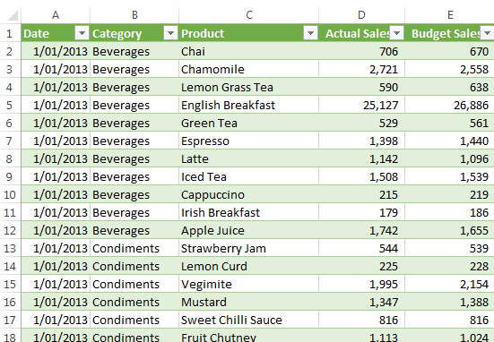
Is your head hurting already? Mine is. Let’s look at an example of when you might use a Calculated Field because it’s really not that complicated; below is my Actual and Budget sales data which is begging to be Pivoted. I’ll create an Actual vs Budget variance report. But wait, I don’t have a ‘Variance’ column:
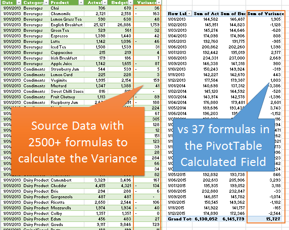
I could add another column in the source data above and calculate my variance for each row of data and then sum it up in my PivotTable, or … drum roll….I could just add a Calculated Field to my PivotTable.
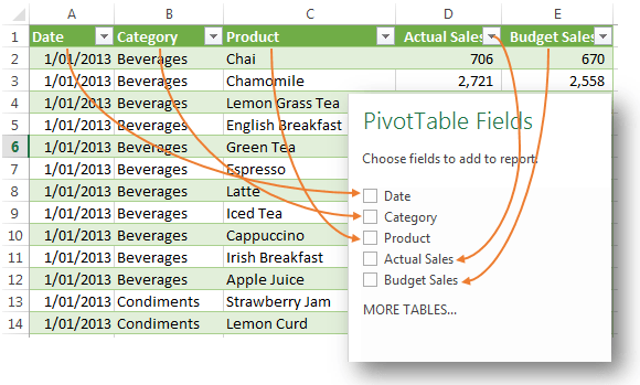
Tip: Here’s how I visualise Calculated Fields; Your PivotTable Field List is simply a list of all of the column labels in your source data (as you can see below), so I like to think of adding a Calculated Field as an alternative to adding another column in your source data.
Whatever you can do in a column in your source data you can do in a Calculated Field…well almost. Don’t hold me to that as I haven’t tested every scenario!
Calculated Fields vs Formulas in the Source Data
Quite simply, formulas in your source data are Full Fat Formulas and formulas in Calculated Fields are Fat Free Formulas!
Full Fat Formulas
Sure it’s easier to just add a simple =E2-D2 formula in cell F2 of the source data then copy it down column F and let the PivotTable add it up, however it’s not the most efficient use of your Excel resources.
You see, if you add that simple formula to column F it gets calculated for every row, and in large files that can result in your file having a MB blowout which means you could end up with a FAT FILE.
Fat Free Formulas
Whereas if you add that calculation to your PivotTable as a Calculated Field Excel only needs to make that calculation when the PivotTable calls for it, and only to the level of detail seen in the PivotTable. That’s why I call them ‘Fat Free Formulas’.
So if your file needs to go on a crash diet simply feed it some Fat Free Calculated Field Formulas and get rid of all the Full Fat Formulas in your source data.
How to add a Calculated Field
Before you can add a Calculated Field you must actually insert a PivotTable, and then with any cell in the PivotTable selected;
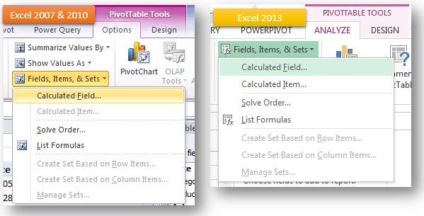
Excel 2007 & 2010: Go to the PivotTable Tools: Options tab > Fields, Items & Sets > Calculated Field
Excel 2013: Go to the PivotTable Tools: Analyse tab > Fields, Items & Sets > Calculated Field
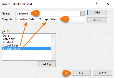
This opens the Insert Calculated Field dialog box:
- Give your new field a name. I’ll call mine ‘Variance’.
- Insert your formula – you can use functions, operators and expressions just like you do in worksheet formulas, with a few exceptions – see the ‘Gotchas’ below.
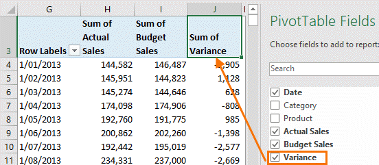
- Click OK (you can click ‘Add’ first if you want but it isn’t necessary), your new field will be in the Field list and in your PivotTable:
You can now use that field in your PivotTable just as you would any other field in the field list.
Modifying and Deleting Calculated Fields
To modify a Calculated Field simply open the Calculated Field dialog box again (remember, select any cell in the PivotTable then on the Options/Analyze tab > Fields, Items & Sets > Calculated Field)
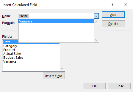
Choose the field from the Name list:
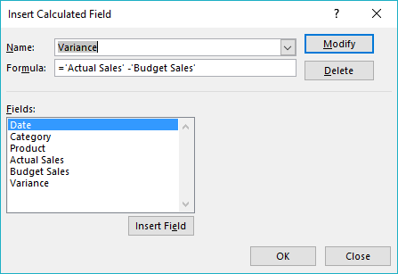
The dialog box ‘Add’ button will become ‘Modify’ and you can make your changes to the formula and then press OK:
Alternatively you can Delete the Calculated Field altogether with the Delete button. Note: this removes it from your PivotTable and the field list so it will no longer be available.
Calculated Field Gotchas
Not compatible with OLAP PivotTables - You can only insert calculated fields in PivotTables created with non-OLAP data sources. For most of us that’s ok since data in an Excel worksheet is a non-OLAP data source.
Can’t use cell references or defined names - Calculated Fields can use operators and expressions (+ - * / > < ^) as you do in other worksheet formulas. You can use constants and refer to data from the report, but you cannot use cell references or defined names.
You can use Functions but you cannot use worksheet functions that require cell references or defined names as arguments, and you cannot use array functions. That means you can use IF, IFERROR etc. but not SUMIFS, COUNTIFS etc. because they require a cell reference for their arguments.
Sometimes the totals will be wonky - Totals aren’t actually totals; every cell you see in the values area for a Calculated Field is the result of the formula. It’s like having the same formula in every cell in the column irrespective of whether the row is a totals row or not.
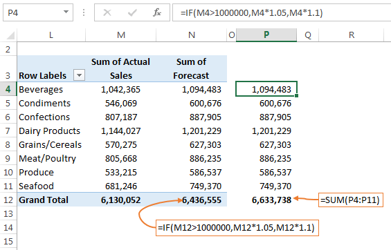
Let’s look at an example. In column N I have a new Calculated Field for my forecast:
The Calculated Field formula is:
=IF(Actual Sales >1,000,000, Actual Sales * 1.05, Actual Sales * 1.10)
Which says, if my Actual Sales for a category is greater than $1m then forecast growth at 5%, otherwise forecast growth at 10%. Probably wouldn’t happen in the real world but let’s go with it.
In the image above we can see column N contains the results of my new calculated field (Forecast) and in column P I have the same formula entered in the cells.
The results are the same until we get to the Grand Total row; cell P12 contains the sum of the values above it, but my calculated field cell N12 still uses the formula even though it’s supposed to be a total.
What to do? You have a couple of options:
- Hide the grand total row.
- Do the calculation outside of the PivotTable.
- Use a Full Fat Formula in your source data and let the PivotTable add them up.
If you can’t live with the above limitations then check out Power Pivot as it can do everything a PivotTable can but isn’t as restricted by most of the above.
And if you've always wanted to master PivotTables check out our Excel Pivot Table course.


Hi Mynda,
I am new to pivot tables and have found your youtube tutorials extremely helpful!!! I have a percentage field in my table called “% Complete” that I would like to translate to a text description based on its value. I am trying to add a calculated field called Status that I would like to use as a slicer but my pivot table shows #VALUE! in the “Sum of Status” in the pivot table. I remove Status from the field list but cannot add it as a slicer. The new Status field has the formula: = IF(‘% Complete’=100,”Complete”,IF(‘% Complete’ =0,”Not Started”,”In progress”)). Any insights would be much appreciated and if there’s a better way to accomplish this, I’m certainly open to it. Thanks, Nick
Hi Nick, calculated fields are typically used to return numeric values that go in the values are of the PivotTable. I’ve never used them for row labels or filters. This calculation is probably better done as a new column in your source data, which you can then reference in a Slicer. If you’re still stuck please post your question on our Excel forum where you can also upload a sample file and we can help you further.
Hello,
Excellent tutorial.
If I need the same custom field over and over again, I have to go in an create it each time?
i.e. I created the calculated field named “% discount” for 2019 on all the items I sell.
I used 2019 discount / 2019 revenue, I want to have this for every year 2020, 2021, etc…. Do I need to create a calculated field for each year?
Hi Daniel,
It sounds like your data isn’t in a tabular format if you’re able to reference a specific year in the calculated item. Probably better to post your question on our Excel forum where you can share a sample Excel file and we can help you further.
Mynda
thanks for the great info :
Can we use the Grand Total in a pivot table to get percentages from each row ?
A= values in a pivot
B= values in a pivot
c= B-A – Which I can do using a calculated field
D = c/ Grand total of B = 25 in this case )
A B C D
1 2 4%
3 6 12%
5 9 16%
7 8 4%
Can this be done using calculated fields in a pivot?
Hi Anwa,
You can only do this with Power Pivot PivotTables because you need to write a custom measure using DAX functions. Regular PivotTable calculated fields cannot reference another field’s grand total.
Mynda
One limitation that derserves recognition is that there is a 255 argument ceiling for functions within pivot calculated fields (formula character length is dependent on the length of the names of the items being referenced not on number of items to be referenced [*what?*why?!!]), which can hinder even the most basic of formulas if the field headers you want to introduce are not in shorthand. Below is a basic example…
Using full description;
“Current Year Q3 Forecast Jan”
=28 Characters
If we want to simply add Jan to Dec we would have:
28*12 months= 336 Characters (Not Possible)
Using Shorthand
CY Q3F JAN
=10 Characters
If we want to simply add Jan to Dec we would have:
10*12 months= 120 Characters (Possible)
Trying to introduce nested formulas into pivot calculated fields almost always fails because of this character limitation.
Even if all of your field headers are in shorthand you can still face this issue as 255 characters is small and arbitrary, and is the reason I rarely bother using pivot calculated fields even though it is a cool feature.
They could be so much more powerful if they removed the charcter limitation, I recall this limitation was on all in cell formulas back in the 90’s meaning nested formuals were no where near as powerful as they are today, given the formula character limit for in-cell formulas is now 8,192 characters, why is this not applicable within this function? *Scratch head*Sigh*Microsoft are awesome!
Anyone else frustrated by this character limit?
Anyone know how to overcome it?
Hi Stuart,
The only way to solve it, if you cannot make the field names shorter, is to try to make all these calculations in your source data.
Until Microsoft removes this limitation, there is not much we can do, unfortunately.
Catalin
How can I use Date data in my Calculated Field = IF(AND(IP>=12000000,’Submited Date'<"01/17/2017"),1,0)? seems it does not work (Submited Date is date column)
Thanks in advance
Hi,
Can you please upload a sample file to our Forum (create a new topic)? Dates can be tricky, it’s important to see what is in that column.
Mynda – nice tutorial, thanks. Question – I’ve created a pivot table using the Relationships option, and this causes the Calculated Field option to be grayed out. Does the use of Relationships automatically put the data in the OLAP category? If so, is there another option than adding a formula to one of the source data tables?
Hi Mike,
‘Relationships’… do you mean you added multiple tables to Power Pivot/Data Model and created relationships? If so then you need to use Power Pivot to create a DAX measure as opposed to the regular PivotTable Calculated Fields.
Kind regards,
Mynda
Option 4: Use a Full Fat Formula in your source data, then copy/paste special values with that result, then make a PivotTable. .
Nice tip, Jeff. Great if you don’t add any new data to your Pivot source.
I seem to recall reading a thread somewhere recently where it was advised to use full fat formulas in the source data rather than calculated fields on really big pivots because of the extra processing overhead required by Excel to create calculated fields on large datasets. I think again it was due to the fact that Excel has to calculate values for every row. Can’t recall where I saw it.
Re your comment “Great if you don’t add any new data to your Pivot source” , I used to deal with monthly raw data that had to have additional information mashed up with it via lots of really intensive array formulas that categorised the items based on partial text strings contained within them. I had something like 10 calculated columns containing those formulas, and a data source size of a couple of hundred thousand rows, and growing every month.
Needless to say this caused significant delays when reopening the file. Needless delays, because nothing about the old data – or the lookup tables that the array formulas were referencing – ever changed. So even though the lookups on all that historical data got recalculated when I opened the file next, they all returned exactly the same answer as they had the last time I closed the file. Indeed, they retured exactly the same result as they did the day they were ‘born’. That is, the day I first put their associated raw data into the file and then copied the formulas down.
These are what I term ‘one-shot formulas’. We need them to provide an answer, but we can guarantee that once provided, that answer is never going to change. So we really don’t need them hanging around anymore, and we certainly don’t want them to recalculate each and every time Excel does a full recalculation.
So I wrote some code that turned any formulas in my table apart from the very first row into values whenever new data was added to the table. Why leave the first row blank? Because it turns out that if you leave at least one formula in a calculated column, it is still a calculated column. Meaning any time you put new data below the table, then when the table auto expands to fit, the blank cells in those calculated columns still get automatically populated with the calculated column formula.
So again, all I had to do was turn those calculated columns back to values (except for the very first line, which meant those Table Column Formulas were still lurking there just waiting for new data).
End result: no full fat formulas, no calculated fields in pivots neither. (Not that I could have used Calculated Fields in this case anyway). And new data got processed automatically without any problems: first it gets given temporary fat formulas to work out the associated values, and then those fat formulas were then turned to hard-coded values in the blink of an eye.
Good points, Jeff. I think to sum it up:
1. If your source data is enormous and Excel is struggling use your ‘one-shot formulas’
2. If your file is getting slow and big then try replacing full fat formulas with fat free ones.
3. If your file is small and running fine you can use any formula you like!
Mynda
Extremely well explained article.
Hats off to Miss T again for another first class post. Thank you 🙂
Thank you, Pratish 🙂
Nicely explained!
There are some cases that Calculated Field is required, even though we have that field in the source data.
Riding on you example, if the variance is in % and we already have that in the source data. We cannot use the field in the Pivot as it will never give meaningful data.
Another example could be rate, e.g. mph/hour.
Simply put, we cannot just average the average. 🙂
Cheers,
Cheers, MF. Good point about the average of averages 🙂