How to Insert Subtotals in Excel

The Subtotal tool in the Outline group on the Data tab of the ribbon automatically inserts subtotal formulas and grand totals for a column or columns. Excel subtotals can be SUM’s, AVERAGE’s, COUNT’s, MIN, MAX and more.

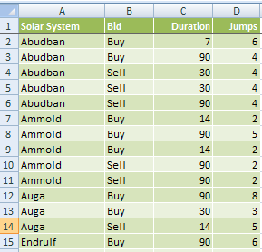
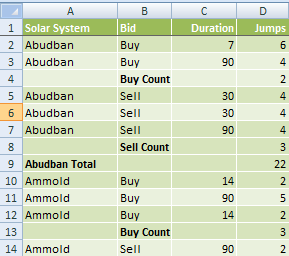
This tool can give you valuable information in a few clicks, transforming your data like this:

How to Format Your Data

First make sure your data is laid out in a sorted table; i.e. the columns you want your subtotal based on must be sorted, like in the example below column A & B are sorted. It must also have column labels, also called a header row, and no blank rows or columns.

Note: You cannot use the Subtotal tool with data formatted in an Excel Table. You need to convert it to a range first.

Insert Excel Subtotals

Using the data below we’re going to insert a subtotal that SUM’s the ‘Jumps’ column at every change in the ‘Solar System’.

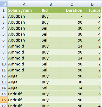
First select a cell anywhere in your table. Then on the Data tab in the Outline group, select Subtotal.

The window below will open.

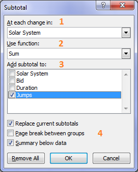
1.       Here you can select the column you want your subtotals based on by choosing from the ‘At each change in:’ list. We’ll select ‘Solar System’.

2.       Select what type of subtotal you want inserted in the ‘Use function:’ list. You can choose from SUM, AVERAGE, COUNT, MIN, MAX and a few more. We’re going to select SUM.

3.       In the ‘Add subtotal to:’ list you can select which columns you want summarised. We’ll select ‘Jumps’ but we could also select the ‘Duration’ column as this has values that can be summed.

4.       You can then select from the check boxes:

• Replace current subtotals: Handy if you’ve already inserted some but you want to change them.
• Page break between groups: Useful for printing your data.
• Summary below data: This inserts the subtotals at the bottom of each change in data. Un-checking this inserts it at the top.

5.       Click OK

Our table now looks like this:

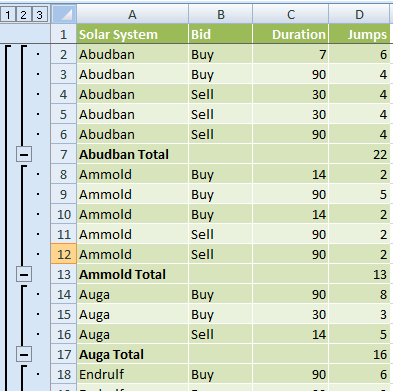
You can see they have been inserted at the bottom of each change in Solar System and notice now you have some new buttons added to the side bar on the left.

These buttons allow you to hide and unhide the detail rows. You can either click the outline symbols or the + and – symbols to expand and contract the rows.

Clicking on level 2 shows the Subtotal rows only, like this:

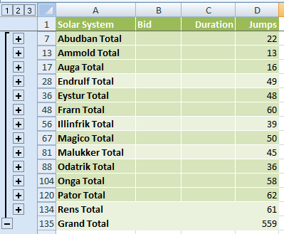
Or you can click on the + and – buttons to hide and unhide individual subtotals.

Clicking on level 1 shows the Grand Total only.

How to Nest Subtotals

Taking the example above, let’s say we want to add a subtotal at each change in the Bid column so that we have a subtotal for the ‘Buy’ items and a subtotal for the ‘Sell’ items.

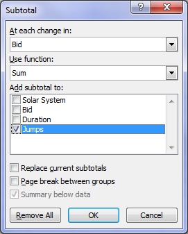
To do this we follow steps 1 to 3 above, and we un-tick the ‘Replace current subtotals’ check box like this so that they are added to the table:

Now our table looks like this:

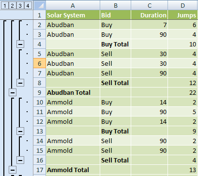
You can see we’ve now got 4 levels in our outline, and we have additional subtotals inserted in the Bid column to total the Buy and Sell items.

We can keep on nesting subtotals and also change the function thus adding more levels to your outline. For example we’ll add at COUNT to our Bid Column like this:

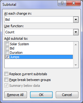
And now our table has 5 outline levels and looks like this:

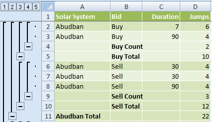
NOTE: I’ve added this fifth level for demonstration purposes, however bear in mind that there will come a time where your table is simply too busy and other methods of summarising your data would be better.

TIPS:

1.       The subtotals are actually formulas and therefore recalculate as you edit the data in your table. Assuming your workbook is set to automatically recalculate.

2.       The grand totals are calculated from the detail data, not the subtotals. Therefore if you insert an Average the grand total will calculate the average for all of the data.