Learning how to customise a cell format in Excel allows you to not only format your data the way you want, but in some instances it can save you time.
Before we dive in you need to know that despite how the text appears after you’ve set your custom cell format, the underlying value is unchanged for the purpose of formulas and calculations.
How to enter an Excel custom cell format
Select the cell/s you want to format then open the Format Cells window.
- The quick way just press CTRL+1
- Or the way most people do it is to right click and select ‘Format Cells’.
- On the Number Tab select Custom from the Category list.
 |
Note: It’s handy to have the text you want to format in the cell before you press CTRL+1 because Excel will give you a sample view of what the text is going to look like in the Format Cells window, so you can see before pressing OK, if it’s what you want.
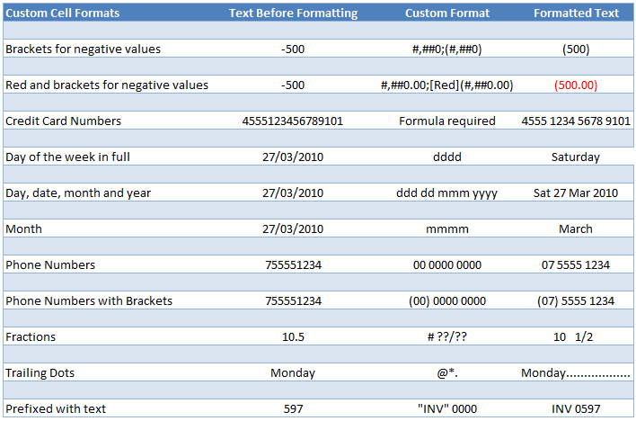
How to make your cell formats look the way you want
| Custom Cell Formats | Text Before Formatting | Custom Format | Formatted Text |
| Brackets for negative values | -500 | #,##0;(#,##0) | (500) |
| Red and brackets for negative values | -500 | #,##0.00;[Red](#,##0.00) | (500.00) |
| Day of the week in full | 27/03/2010 | dddd | Saturday |
| Day, date, month and year | 27/03/2010 | ddd dd mmm yyyy | Sat 27 Mar 2010 |
| Month | 27/03/2010 | mmmm | March |
| Phone Numbers | 755551234 | 00 0000 0000 | 07 5555 1234 |
| Phone Numbers with Brackets | 755551234 | (00) 0000 0000 | (07) 5555 1234 |
| Fractions | 10.5 | # ??/?? | 10 1/2 |
How to save time with Custom Cell Formats
1) From time to time I create a reference sheet like a contacts list, an index or even just a list of items like the one below using the custom cell format @*.
 |
Because the text in the first column is often different lengths it can be hard for the eye to follow across. In these cases I like to use trailing dots to help the reader.
I wouldn’t dream of manually entering the dots but since I can create a custom format it’s worth it, plus I think it looks more elegant that using borders for this purpose as they can get a bit busy.
The custom cell format for trailing dots is @*. When you type in your text Excel will automatically enter the dots to fill to the end of the cell.
Tip: You’re not just limited to dots. You can have ---- or **** or ____ or almost anything you want. Just replace the dot in the custom format with the character of your choice.
2) The other custom format I use regularly is prefixing my data with text. For example, I keep a record of our invoices and instead of typing ‘INV’ before each number I enter I use a custom cell format like this: “INV” 0000
Then when I type in 597 Excel converts it to INV 0597.
Tip: Replace INV with different text to suit your needs. It might be PO for purchase order, or any other text you can think of. Or make the text a suffix by changing the custom format to 0000 "INV".
Remember that even though the text appears to be INV 0597, for the purpose of formulas it’s still just a number 597.

Formatting cells for credit card numbers
You might be thinking you can use a custom format of 0000 0000 0000 0000 for credit card numbers, but you’ll find that it will only work for cards where the last number of the card is a zero! Try it out and see for yourself.
The workaround is to use a formula. This requires entering the number in one cell, and then in another cell you need to enter the following formula (assuming our credit card number is in cell A1):
=LEFT(A1,4) & " " & MID(A1,5,4) & " " & MID(A1,9,4) & " " & RIGHT(A1,4)
Note: I’ve added spaces in the formula for clarity.
Some explanation:
- The LEFT, MID and RIGHT returns text from a specified position in a cell.
- The ampersands ‘&’ join text together
- The “ “ adds a space between each group of text
[UPDATE] - You can also use this custom number format for credit cards and long phone numbers:
[<=99999999999]##########;#### #### #### ####
Thanks to MF for sharing that tip.
Enter your email address below to download the sample workbook.

Greetings and thanks for a very informative site.
I tried the custom format mentioned as an update above, credited to MF:
[<=99999999999]##########;#### #### #### ####
It worked as expected in Excel 2010 but in Excel 365 the digits are grouped in threes and I haven't been able to find out why. Update in Excel, or could it be an options setting?
I have 365 and the digits are correctly grouped for me.
Thanks for the quick reply. I’ll let you know if I get to the bottom of it.
Hi Mynda,
after reading your note that MF’s format worked in 365 for you, I looked further afield, to the Windows Regional settings. I had English (UK) set, and in the number format dialogue I had defined a space as the separator and grouping in threes instead of the standard comma separator for that region. After I reset the number formats to the default for the region and applied it, then restarted Excel 365 MF’s custom format was no longer changed by Excel, and the format worked as expected.
Keep well!
Glad you figured it out, Christo!
P.S. It seems that my Excel 365 won’t accept
[<=99999999999]##########;#### #### #### ####
as a custom format. As soon as I hit OK the dialogue closes and the numbers are displayed in groups of three; if I reopen the Custom Format dialogue the format I defined has been changed to
[<=99999999999]##########;# ### ### ### ### ###
I wonder if it’s a regional/locale issue. My locale is set to English.
P.S. to mine of a couple of minutes ago. I’ve just seen your reply about regional settings – I think it was my customising the English(UK) settings that was the problem. Thanks again.
I use the same customer format each day. ‘###############’, Is there a way to add this custom format in excel so that it is in the custom drop down list permanently? Not just for the workbook I used the day before, but for every workbook I open, so I don’t have to create it for each and every workbook I use?
Hi Chris,
You can save the format to your default Excel workbook.
Mynda
Do I use the SUMIFS way on data file?
Hi,
Sorry I don’t understand your question, can you please rephrase it and provide as much information as possible.
Regards
Phil
How to made text between bracket in one cell
ex: in one cell –> ( tr )
bracket on left and right, and text on center, all in one cell
Custom cell format:
(@)
The @ symbol represents text.
Mynda
I like to work on EXCEL efficiently.
I find it very helpful
I want to know how to calculate my times for work. This is hard to understand.
Hi Nicole,
This tutorial explains how dates and times work in Excel. If you’re still stuck after that, please post your question in our forum where we can help you further.
Mynda
you shouldnt be encouraging people to capture credit card numbers in Excel documents as that causes big problems with security and PCI compliance.
Hi Chris,
I’m not sure I said anywhere that people should capture credit card numbers in Excel. I just told them how to format them if they wish to.
Some people use Excel to record their own credit card numbers, which doens’t breach PCI compliance. Now I’m not saying I recommend they do that either, but if they want to do so that’s up to them, and at their own risk.
Mynda
I have difficulty with the custome format…I cannot make @*. I only can find @. pls help.
Hi Albert,
The format is entered as a custom number format. You won’t find it in the list.
There are 3 characters in the format like this: @*.
You choose ‘Custom’ from the Category list and then enter the format in the ‘Type’ field.
Let me know if you still have trouble.
Mynda
I need a help for converting numbers to text. I have a data in outlook with 19 to 20 digit along with some other text fields in vertical format. While I copy paste this data in excel these 19 digits are pasted as numbers and they are changed to 000 at the end or I get a number like 65962656+000. For this I have to again copy the data from source and put an apostrophe before pasting the 19 digits to show as text.
Can we have a solution here to save my extra effort of putting an apostrophe?
Have you tried to format the destination range as Text, then paste source data as values? This should stop excel from automatically convert numbers. When excel converts a number, only 15 digits are accepted, the rest will be replaced with 0, changing the destination format to text should be enough.
I would like to create an Excel spreadsheet to calculate my nightshift working hours subtracting my unpaid break in minutes. running horizontally. Thanks.
Hi Joe,
Can you upload a sample file with your data on our Forum?
It will be easier to help you when we know your data structure, most of the times there will be differences between when you mean and what we understand from your explanations.
Thanks for your understanding
Catalin
Somewhere I saw how to build this custom format ▲_(* #,##0.00_);[Red]▼_(* (#,##0.00);_(* “-“??_);_(@_) but now I cannot find where I saw this. Unfortunaetly I did not write down how I constructed the custom format. Can you direct me to where I can find this. It is not part of the custom format blog posting. Thanks
Hi Michael,
I’m not sure where you saw that format. It might have been in my Excel Dashboard course. I wrote a comprehensive guide to Excel Custom Number Formats.
Mynda
Great site, I have a custom date format formula I need help with. I need to print timesheets monthly for weekdays only, and have formatted the cell to read the date in the ‘ddd’ format (Mon, Tue, Wed, etc.). I have tried this formula to skip the weekend dates =IF(‘1’!A1=”Fri”, ‘1’!A1+3, ‘1’!A1+1). I can’t get it to read the ddd format as “Fri”, it just reads the statement as false and adds 1 day to the date in cell A1. Any idea on how to write this formula without having to create a VLOOKUP?
Hi Mike,
The date in A1 is a number, as you already know. There will be a mismatch if you try to compare a number to a text, both items should have the same data type. Because “Fri” is a text, you have to convert the number from A1 to a text. The easiest way is using the TEXT formula: =IF(TEXT(’1′!A1,”ddd”)=”Fri”, ’1′!A1+3, ’1′!A1+1)
This way, you will have both terms with the same data type, and you will be able to compare them.
Cheers,
Catalin
Catalin, your suggestion worked. I knew there was something missing from my formula that was causing it to be misread. It hadn’t occurred to me to try the TEXT formula.
You are the best!
Mike
Hi Mike,
it’s always a pleasure when we can help 🙂
Cheers,
Catalin
Absolute cracker
Thanks, Jeevan! 🙂
I am looking to add 5 hours to a CDT number in the format dd/mm/yyyy hh:00 to get a GMT value. Can you help?
Hi David,
The format is irrelevant, because any date/time represents a number, it can be displayed in many ways, but it’s still a number, days are integers, and hours are subunits. 1 day represents 1 integer, so 1 hour is 1/24. To add 5 hours, simply add 5/24 to your time:
=A1+5/24
Cheers,
Catalin
Hi there, I need some help with a formula please.
I want to set up a time sheet with only time in, time out, hours worked subtracting 1 hour for lunch and then at the end of the month calculate the hours, but display as 30 min in stead of .50
Should look like this
Time in Time out Daily hours Monthly hours
09:30:00 AM 03:00:00 PM 05:30:00 5.30
09:30:00 AM 03:00:00 PM 05:30:00 11.00
Looking forward to hearing from you soon,
Hi Rene,
Displaying time in decimal system style format is confusing, and may be wrongly interpreted… 5.5 is in decimal system, 5:30 is in sexagesimal system, but both mean the same thing: 5 hours and a half.
If you still want that, you can format Monthly Hours as time format, with this custom format: [h].mm
Catalin
Great information on this page, thanks. Hi have a question I can’t find any answer to. You can use the custom cell format to convert digits/numbers to letters or words like:
[=1]”yes”;[=2]”No”
I wont to do the opposite! In the cell the operator makes his entry I want to check if the entry is “x” and in that case replace the “x” with a number. If the operator enters a number I want to leave that as it is. If possible I don’t want to use VBA! Any solution you can think of?
i’m afraid that’s not possible, the text operator (@) is limited. Only VBA can be used…
Catalin
I accidentally deleted a custom cell format that essentially makes a cell a blank rather than a “0” (last choice in the custom Type).
How can I get that blank back?
Hi Alan,
Custom number formats are made up of 4 components:
Positive values ; negative values ; zero values ; text
Not all values need to be stipulated in a custom number format. e.g. you can just stipulate positive and negative values and zeroes will be treated as a positive value.
If you want to hide zeroes then you need to make sure the third argument is empty e.g.:
0.0;-0.0;;
The above format will format positives and negatives but because the zero format is empty they will not be displayed on your worksheet.
Let me know if you get stuck.
Kind regards,
Mynda.
I have my sales data in Thousands , but I want to show it in millions in the summary report and also in the charts for monthly meeting, – is it possible without converting the original data into millions
Hi Saurav,
You can right click on the axis values, choose Format Axis, under Axis Options, select Display Units: – Millions (usually, the default in None)
A value of 8000, for example, will be displayed as 0,008 Millions.
Catalin
This tip came a just the right time. I was struggling with custom formatting for something very similar just yesterday.
Thank you for the tips. They really make our lives easier.
Great! Glad we could help, Sherry 🙂
Hi,
How is the normal 10 digit mobile phone number formatted, as in 0400 600 800, please? (Group of four digits, space, group of three digits, space, group of three digits)
Hi Frank,
Right click the cell, Format Cell–>Custom, and in Type section, type: (0000) 000 000 with or without the brackets, as you like.
Catalin
Thanks Catalin,
I’ve already tried that and it says “cannot use the number format typed”. I have Office 2010 (and hate it).
I also use Office 2010, and it worked without problems. Use “” if you are typing other characters than the brackets or spaces. Try this: In Special formatting category, you might have a Phone Number preset.
Thanks, it worked. The Excel help from MS is woeful.
I would like to be able to enter a decimal number into a cell such as 25.5 and see the format converted to feet and inches as follows: 25′ – 6″
I have found a custom format that goes as far as 25′ – 6/12″
Is there some way to truncate the /12 from the above format?
Thank you,
Mike
Hi Mike,
Unfortunately, the custom formats are limited, there is no way to do that…
All you can do is to enter decimal values in a column, and use formulas to format as you like in next column.
Cheers,
Catalin
hi mynda ; perfeact .Cheers
Thanks, Mano 🙂
I am using the trailing dots in 2 excel sheets. The first one worked flawlessly using the @*. method. The 2nd sheet is not being cooperative. It is working for some of the cells, but not all of them. The cells all have the same basic content – numbers or numbers and letters – I don’t see any visible reason this would not work, and when I click on the cells not working the formula bar shows the text is in the cell, and clicking on cell properties indicates the formatting is applied.
Hi Dan,
Sounds strange. Are you able to send me your Excel file via the help desk so I can see what you’re working with?
Cheers,
Mynda.
I need to set up a spread sheet to show 72 hours of an advanced date of meetings. Example: If there is a meeting set for Monday at 8:00 a.m. I would need all documents 72 hours prior to that day and time. How would I calculate this?
Hi Sharon,
In your meeting time cell (say A2) enter the date and time as follows:
20/05/2013 8:00 AM or if you use mm/dd/yyyy date format enter it as 05/20/2013 8:00 AM
Then in cell B2 enter this formula:
=A2-3
3 is 3 days or 72 hours.
Kind regards,
Mynda.
Hi okay, i’ve searched around and can not find anything on this scenario. I have 12 digits, the first two need to be surrounded by parentheses and are either a space w/ one letter, two letters, or two numbers; the rest are all numbers w/ dashes between some of the numbers. I would like a formula where it will allow the first two digits to be either the letter or number. I enter all 12 digits in the cell and the formula produces either…
(AL) 05-10-451-013
(88) 20-12-376-101
(K) 25-14-152-078
a formula for the cell would be extremely appreciated, if even possible. Cathy
Hi Cathy,
="("&LEFT(A1,SEARCH(" ",A1)-1)&") "&RIGHT(A1,LEN(A1)-SEARCH(" ",A1))Where your value is in A1
Kind regards,
Mynda.
Its really a usefull information. THANKS a ton for it.
You guys are really doing a tremendous job to promote advanced excel. Many people use this incredible thing just for entering the data and dont know how to use any of the remarkable formulae.
Keep the good work going. Thanks…
Hi Shazif,
On behalf of Mynda,
You’re welcome!!!
Carlo
1. The custom cell format for trailing dots is @*. When you type in your text Excel will automatically enter the dots to fill to the end of the cell
not very clear, I typed – ansbgv in left cell then gap few cells on right then typed gjkhuy. I wanted to link between ansbgv & gjkhuy with trailing dot – how?
2. The other custom format I use regularly is prefixing my data with text. For example, I keep a record of our invoices and instead of typing ‘INV’ before each number I enter I use a custom cell format like this: “INV” 0000
Then when I type in 597 Excel converts it to INV 0597 =
Which tools need to be used to convert?
Thank you
Hi Aparna,
Regarding Solution for number 1, I am sorry but I don’t think it was meant for linking two words in a cell. That is why
it is called , as you said, ‘trailing dots’.
Regarding number two I don’t understand what you want here. You stated perfectly your case and it seems you have your
answer already. So what do you mean by “tools to convert”?
Cheers,
CarloE
I want to be able to type in numbers from 1 through 59 and the cell automatically formats to read 1 min. through 59 min. i do this with _(#_*”min.” as a custom format.
the problem arises when I type in 60 I want it to display as 1 hr.
I don’t want formulas in the cells.
any calculations need to be invisible or possibly handled as a VBA for the workbook.
I want to be able to type in 65 and have it display as 1 hr. & 5 min.
please send answers to [email protected]
Markus,
As much as we wanted to help you,
VBA is outside the scope of services/support
we are currently providing.
Please do come back when we will have VBA services
soon.
Cheers,
CarloE
thanks for your tips
Hi Lenin,
You are very welcome,
On behalf of Mynda.
Cheers,
CarloE
Regarding the sixteen digit credit card number, it is not the fact that the last number has to be zero, it is that Excel uses 15 digit numbering.
Try it with a twenty digit number, the last five digits will translate to zeros.
Cheers, Gerry. This is why when the last digit is in fact a zero it ‘appears’ to work.
It’s Fantastic, Thanks a lot.
Cheers, Ali 🙂
Hi ,
thanks a lot for your excel formating content. i have a phone field some time it will have 10 digit value (e.g.7877988334) some time it may have phone field with the country code ( e.g. (+91) 7877988334 ). how to create the format to support both of them.
waiting for your reply,
with regards
Solomon
Hi Solomon,
You can’t have one custom format that handles different scenarios.
Kind regards,
Mynda.
Inspired by the last comment, try this in the custom format:
[<=99999999999]##########;(+##) ##########
If your input is 12 digits, the latter format applies.
Thanks, MF. You’re a genius 🙂
I will have to share this magic with our members.
Likewise you can modify it for credit card numbers:
[<=99999999999]##########;#### #### #### #### Cheers, Mynda.
Thanks for your kind word!
I just learn from all of you.
Awesome, as usual. I daily just wait for your article.
Another way to enter the credit card number is to add – ‘ ( key on the left side of enter key). The number is stored in text, However this is on the best way.
thanks
🙂 You’re welcome.
Realy a greate tutorial, I find this tutorial very helpful,
Cheers, Asghar 🙂 Glad you liked it.
Some great tips I had not come across before!
Thanks Jenny 🙂
Thanks, it was just what I needed.
You’re welcome Melanie. Glad we could help.
Great website guys 🙂 This kind of help is worth its weight in gold! Well done to you, it should go really well! Sherree xo