Here are some easy solutions to Excel cell formatting frustrations that I get asked about all the time.
Enter your email address below to download the sample workbook.
1. Force text to wrap to the next line
How often do you add extra spaces between your text to force it to wrap just the way you want, only to change the column width and to have to do it all over again? It’s frustrating and a waste of time.
Thankfully there’s a better way to get your text to wrap to the next line in Excel. Simply press ALT+Enter after each word you want to wrap. This forces the text onto the next line.
Tip: don’t add a space after the last word on each line otherwise it won’t be centered properly.
 |
2. To Merge & Center or To Center Across Selection
How often do you get that error message ‘Cannot change part of a merged cell’?
Or have you ever been in the process of highlighting a series of cells and all of a sudden your mouse scrolls over some merged cells and BAM, the area you’re highlighting is three times the size you want?
I’m sure you’ve had moments where you’re cursing the merged cells for one reason or another. Well there’s a better way to merge cells too.
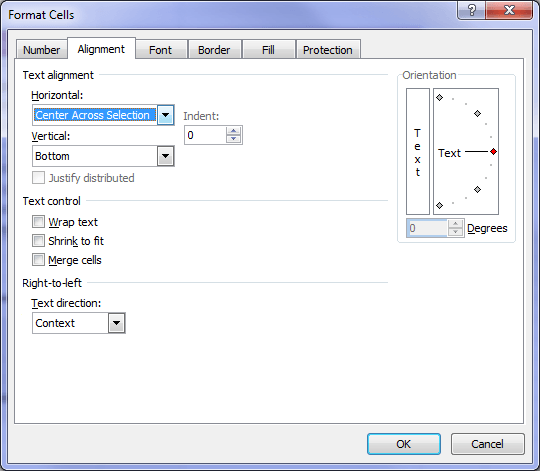
And it’s called Center Across Selection. To use Center Across Selection:
a. Enter your text in the left most cell that you want your heading in
b. Highlight the cells you want your heading centered across
c. CTRL+1 to open the Format Cells dialog box
d. On the Alignment Tab select Center Across Selection from the Horizontal drop down list
 |
The differences between Merged Cells and Center Across Selection is:
- Merged Cells converts multiple cells into one big cell.
- Center Across Selection keeps the underlying cells as individual cells and simply centers the text for you.
The limitation of Center Across Selection is that in can only center across one row because it’s simply horizontal text alignment. Ah, but there’s a solution to this if you really want your headings to straddle more than one row.
3. Excel Shapes As An Alternative to Merge & Center
 |
Shapes can be found on the Insert tab under Illustrations.
a. Choose the shape you want
b. Drag the mouse pointer to draw the shape the size you want
c. Format it using the new ‘Format’ tab that appears when the shape is selected
d. Write your text in the shape and format your text as you normally would
You can see in the example above that the shape appears to be floating above the cells. This is partly because it has a shadow effect, but also because it actually is floating.
You can still type text underneath the shape (a handy place to put information required for the worksheet, but not required for the reader of the report).
I’m going to do a tutorial dedicated to Shapes, so I’m not going to say much more here. But needless to say, shapes are fast becoming one of my favourite features in Excel for making my reports look professional, while at the same time eliminating the restrictions of Merge & Center.
4. Bonus Excel Cell Formatting Tip – Fill
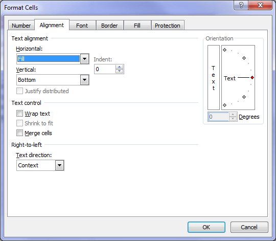
While fiddling with the cell formatting options I stumbled upon ‘Fill’ in the Alignment Tab.
 |
You can see in the formula bar that I’ve only typed in ‘Fill’ once and Excel has repeated it across the selection. Note: I actually typed in ‘Fill ’ with a space after it so you could read it without going cross-eyed! Mind you, I’m not sure it helped all that much 🙂
 |
At first I couldn’t think of why I’d use the Fill formatting style, but then I thought it would be handy to use it as a dot leader.................................................like this.
Or a star leader ********************************like this, and so on.
Of course this would require you to have at least three columns. The first one with your text in it, the next one with your dots or stars, or whatever you choose, and the third one with your text in.
Alternatively you could use one of the custom cell formats in one of my previous tutorials.
I must say it has been quite a challenge to spell 'center' with an 'er' rather than an 're' since I speak English English, not American English. So in case you're wondering, I did this simply to be consistent with the spelling in Excel 🙂
Got any formatting tips you'd like to share? Please tell us in the comments below.


Mynda l am getting a lot of help in excel from your on line training hub.
Many thanks always
You’re welcome, Watson 🙂
Can anyone assist with UNDOING or REMOVING a forced wrap command (ALT+ENTER) from a string of text? We have a data base that outputs the entire customer address into one cell (up to 4 lines) and I’m trying to break out zip code and state. I think the first step is unwrapping the data string.
Thanks for any ideas!
Hi Mario,
There are two ways:
1. Do a Find & Replace of the character. To do this press CTRL+H to open the Find & Replace dialog box > In the Find field hold down the ALT key while you enter 010 > in the Replace field enter a space or other character as you wish.
2. Use the SUBSTITUTE function. =SUBSTITUTE(A1,CHAR(10),” “) where A1 contains the text you want replace, CHAR(10) is the carriage return you want removed and ” ” is replacing it with a space.
I hope that helps.
Kind regards,
Mynda.
Came across this blog after unsuccessful search for an answer to the following. I see that the last post was 2011, but thought my question might be relevant.
I use merge cells and word wrap to format text in a large, multi-sheet workbook. I often have to type a series of words, like the type of material, separated by “/”, e.g. metal/glass/composite/…. . Word wrap puts the whole sequence on a new line if it does not fit on the current line. How can I get Excel to break the line at the “/”? My client does not want “metal / glass / composite / ” and entering a space (or Alt+Enter) to create a break at the right spot would be tedious even if I could do this, but I can’t because Excel does not print the same as it formats on screen so I don’t know where to put the space to get the correct wrapping (unless I flip back and forth at each occurrence to see it in print preview – even more tedious).
Thanks for your help.
Frank
Hi Frank,
Thanks for your question. If you force a break using ALT+ENTER it will print the same as it looks on the screen. I’m not aware of any custom cell format that will wrap text at the “/” characters, sorry.
If you force a carriage return using spaces that’s when you get inconsistent views between printing and screen. ALT+ENTER is your solution, albeit tedious.
BTW, the last post was last week. You can see the latest posts on the blog.
Kind regards,
Mynda.
thx
This tip is courtesy of Margaret Burt.
For those of you who use Excel on a Mac you can force a carriage return with the Command + Control + Enter keys.
Thanks for your input Margaret.
Thanks Mynda, Looks great I will give it a try and let you know how I go with this. Thanks for the prompt reply.
Jim
CAN ANYONE TELL A NEWBY HOW TO CREATE A CELL FORMULA THAT KEEP THAT CELL BLANK UNLESS DATA IS ENTERED INTO ANY CELL OF A RANGE OF OTHER CELLS IN THE SAME SPREADSHEET? FOR EXAMPLE I WANT TO HAVE CELL A15 STAY BLANK AND ONLY DISPLAY CERTAIN (PRE DETERMINED) TEXT IF DATA IS ENTERED INTO CELLS A1 TO A10 OF THAT SPREADSHEET. I CAN DO IT USING THE IF FUNCTION BUT ONLY TO A SINGLE CELL NOT TO A RANGE OF CELLS.
Hi Jim,
Yes you can, and yes you use an IF statement.
Let’s say your cells (A1:A10) contain text, as opposed to numbers, you could use the COUNTA function to count if any cells contain text. And if they don’t then leave the cell blank, but if they do then enter “your text”. Like this:
=IF(COUNTA(A1:A10)=0,””,”enter this text”)
Translated the formula above reads:
=IF(the number of cells in the range A1:A10 that contain text is = 0, then put nothing in the cell, otherwise put the words “enter this text”)
Note: if cells A1:A10 contain numbers then replace COUNTA with COUNT.
Let me know if that helps.
Regards,
Mynda.
Hi. Re: Force Wrap Text, I must be doing something wrong, because when i press CTRL+ENTER it doesn’t work???
I just googled it, and it’s actuallt ALT+ENTER :o)
🙂 Oops, you’re right. It’s one of those things I do on auto pilot but when I have to think about it get’s all mixed up. I’ve corrected the post. Thanks for letting me know.
thanks, very informative..