Excel Factor 10 Conditional Formatting Painting by Numbers

This Excel Factor entry was sent in by Rob Anderson of Oxfordshire, UK.

Project planning and other tracking worksheets can be enhanced with Conditional Formatting.

Rob uses a clever trick to quickly colour code cells using conditional formatting like columns F:M below:

Remember painting by numbers? It’s a bit like that. Where 1 = blue, 2 = green, 3 = red and so on.

Set up Painting by Numbers with Conditional Formatting

1. Select the cells you want the Conditional Formatting to be applied to.

 

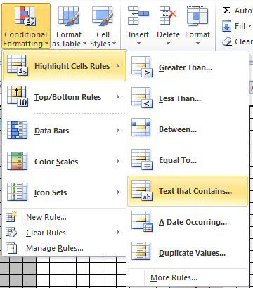
2. On the home tab of the ribbon select Conditional Formatting > Highlight Cells Rules > Text that Contains…

 


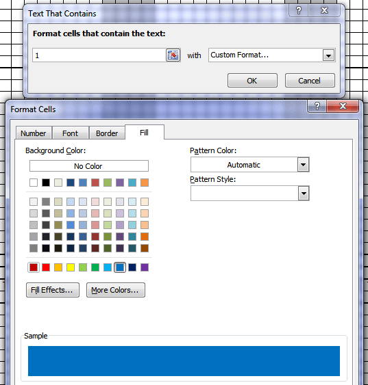
3. Set up your first rule. We’ll do 1 = blue first.

 


Here’s the trick, make sure you set the colour of the fill and the font to the same shade of blue. That way when you enter a 1 in the cell you won’t see the actual number as it will be the same colour as the fill.

4. Rinse & repeat for other number/colour combinations.

Painting by Numbers Variations

• Instead of typing a number in the cell, you can use other characters like */=+ etc, or combinations of numbers and symbols. Simply set up your Conditional Formatting accordingly.
• Use formulas. E.g. If 2 = green then the formula =1+1 will format a cell green. Obviously this is a silly example, and you could do something much more sophisticated with and IF statement, or other formula that reads the results of a cell and returns the relevant value.
• Use a combination of cell fill and symbols to indicate different statuses in the one cell:

 

Thanks for sharing this tip, Rob.

Vote for Rob

If you’d like to vote for Rob's tip (in X-factor voting style) use the buttons below to Like this on Facebook, Tweet about it on Twitter, +1 it on Google, Share it on LinkedIn, or leave a comment….or all of the above 🙂