Finding a Needle in an Excel Haystack

By Harold Graycar XL Numerics Developer of Excel for Customer Service Professionals

When dealing with large tables containing ‘buckets’ of numbers, we often need to find the location of the largest number, the smallest number, etc.

There are a couple of techniques in Excel for doing this:

By eye: using conditional formatting etc.

By formula: using some relatively simple formulas to find the row, the column, and the exact cell address of the largest/smallest numbers.

We’ll be looking at a small table for the examples, but these techniques work equally well for hundreds of rows and columns.

Download the workbook

Note: we’re using Excel table names and range names throughout – it makes the refences so much simpler, and you can follow the details in the example workbook.

1. Conditional formatting – the Heat Map

This method sets up a simple visual method for identifying large and small numbers by applying ‘Heat Map’ formatting to the data:

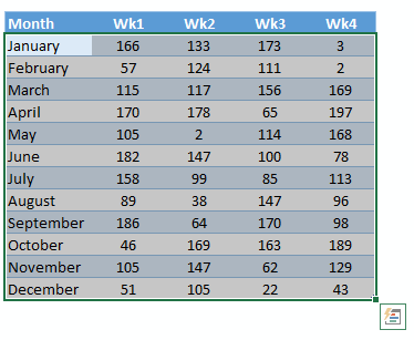
Select the data table you want to format:

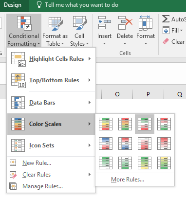
From the Conditional Formatting menu on the Home tab, choose Color Scales:

And you will have a clearly laid out ‘heat map’ with the largest numbers in green, and the smallest in red.  The colours get bolder as you approach the ends of the range, with the middle numbers shaded in white.

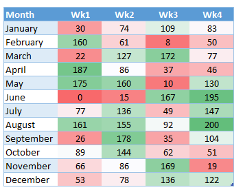
This is a useful technique for looking through the data, but doesn’t give you the ability to work directly with the largest or smallest numbers.

2. Conditional formatting – showing the maximum and minimum

This method sets up a simple visual method to identify the maximum and minimum numbers in the table

Firstly, outside the table, identify the maximum and minimum numbers with formulas:

The cell holding the maximum number is given the range name Cmax, and the cell with the smallest number is given the range name Cmin.

The you can set up two simple conditional formats on your data table

From the Conditional Formatting menu on the Home tab, select New Rule:

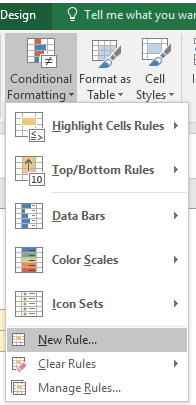
and then ‘Use a formula  . . . ‘

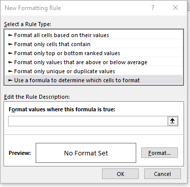
The formula to use looks like this (and you could easily modify it to your own requirements):

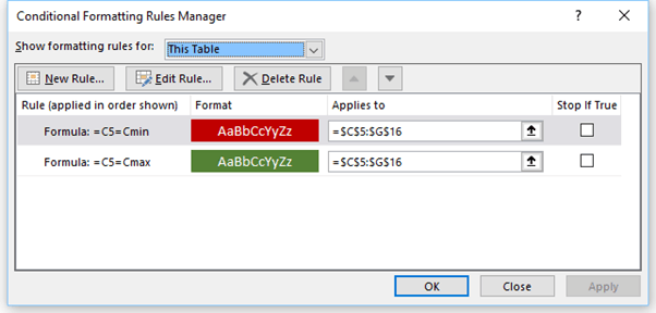
i.e. the maximum number will always be rendered with a green background, and the minimum will be rendered with a red background.

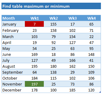
Again, this is a useful technique for looking through the data and directly identifying the largest and smallest, but doesn’t give you the ability to work directly with those numbers.

3. Using formulas to directly find the maximum and minimum

This method uses the MATCH formula to directly address the largest and smallest numbers in the table, and the CELL formula to identify the exact cell address.

Because the method is identical for the largest and smallest, we have set up a drop-down control, using Data Validation to run the method for either the largest or the smallest – you get two methods of analysis for the price of one . . .

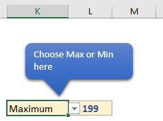
In K7, we can select ‘Maximum’ or ‘Minimum’ by using Data Validation, and the formula in L7 is:

=IF(K7="Maximum", MAX(MyTable),MIN(MyTable))

This cell is then given a range name of ‘Selected’ so that the formulas can easily refer to it.

Now, the main table in which we’re searching for data needs to have alongside it a reference row and a reference column (shown in green here):

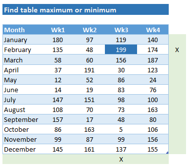
The reference column at right, which has been given the range name ‘RowMatch’, shows the value X where the highest number is located by the formula:

=IF(ISNUMBER(MATCH(Selected,C5:G5,0)),"X","")

The reference row below, which has been given the range name ‘ColMatch’, shows the value X where the highest number is located by the formula:

=IF(ISNUMBER(MATCH(Selected,MyTable[Wk1],0)),"X","")

These values of X are then matched to the table to provide the row, column and full address of the Selected cell (i.e. the maximum or the minimum or the lowest).

The row of the Selected cell is given by                =MATCH("X",RowMatch,0)

The column of the Selected cell is given by         =MATCH("X",ColMatch,0)

And the full address of the Selected cell is given by:

=CELL("address",INDEX(MyTable,MATCH("X",RowMatch,0),MATCH("X",ColMatch,0)))

And of course conditional formatting is used to highlight the Selected cell, using the conditional formatting rule:

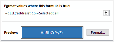
This is the best technique when you need to locate the specific row, column and cell address of the largest and/or smallest number.

It then gives you the data for extracting, comparing and further processing that data.

So we’ve covered three ways in which you can locate the largest and smallest numbers – and some neat formulas based on the MATCH function for extracting the locations of those numbers.

There’s a whole lot more on how to use these conditional formatting and formula techniques in the Excel for Customer Service Professionals course.