One of the nice features of Excel Tables is the banded row formatting, which makes it easier to read and scan your data.
Unfortunately Excel Tables aren’t efficient with large data sets (over 100k rows), but we can replicate the banded rows with Conditional Formatting, and we can toggle it on and off at the click of a button like this:
Download the workbook
Enter your email address below to download the sample workbook.
Toggle Excel Conditional Formatting On/Off
First of all we need a check box or radio button form control. You’ll find the form controls on the Developer tab > Insert:
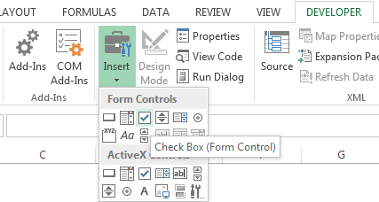
Note: if you don’t see the developer tab click here for instructions on how to enable the Developer Tab.
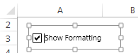
Draw the check box form control onto your worksheet.
To edit the default text hold CTRL and left-click the form control; this will display the pull handles to adjust the size, and you can click inside the box to edit the text.
It is a floating object so you can move it around by left clicking and dragging while the pull handles are visible.
Set the Cell Link: Right-click > Format control
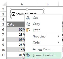
Choose a cell to house the status of the check box. Mine is in cell I3:
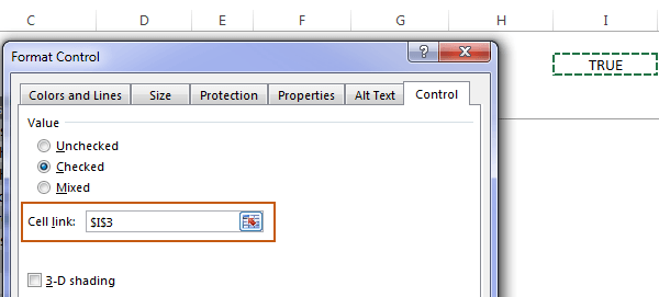
When the check box is checked the cell link, cell I3, will contain TRUE, and when it’s unchecked it contains FALSE. We use this in our Conditional Formatting formula.
Set Banded Rows with Conditional Formatting
To set the conditional formatting we first select the range of cells we want to apply the formatting to. In my case it’s A6:G48.
Tip: I don’t recommend you format the whole row/column as this will just bloat your file. Better to only format the rows and columns that contain data.
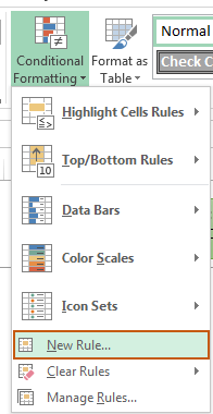
Then on the Home tab > Conditional Formatting > New Rule…:
In the Edit Formatting Rule dialog box (shown below), choose ‘Use a formula to determine which cells to format’:
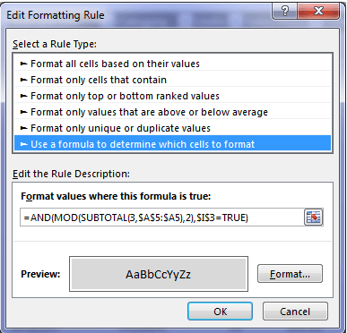
And in the formula field we use this formula:
=AND(MOD(SUBTOTAL(3,$A$5:$A5),2),$I$3=TRUE)
In English the formula reads:
Count the number of visible rows in column A (that’s the SUBTOTAL(3… part, where 3 is the COUNTA function for SUBTOTAL), divide the count SUBTOTAL returns by 2, and return the remainder, (that’s the MOD part), which will always evaluate to either 1 or zero AND check to see if cell I3 contains TRUE
Conditional Formatting formulas must always evaluate to either TRUE or FALSE, or a 1 or 0, which is the numeric equivalent of TRUE and FALSE. A TRUE or 1 will apply the format, and FALSE or 0 hides the format.
To summarise the formula; If the MOD(SUBTOTAL formula evaluates to 1 AND $I$3=TRUE then Excel will apply the format.
Let’s look at the key components of the formula.
The SUBTOTAL function in the formula allows us to apply filters to the table and have the banding automatically adjust so that only the visible/unfiltered cells are banded. This is because SUBTOTAL can ignore hidden rows. Learn more about the SUBTOTAL function here.
We use absolute referencing to tell Excel which cells to reference as the conditional formatting moves through each row. This post explains how conditional formatting formulas work.
The MOD Function:
MOD Syntax:

We use SUBTOTAL to return the number argument for MOD, and the divisor is 2.
You can see it below where I’ve entered the MOD(SUBTOTAL part of the formula in column I:
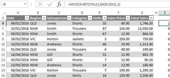
Lastly, we check the value in cell I3 to see if the check box is checked (TRUE), or not checked (FALSE).
Tip 1: Column A must not have any blank cells, otherwise the SUBTOTAL count will be wrong. You can choose a different column for SUBTOTAL, just so long as there are no empty cells.
Tip 2: If you don’t need to filter your data then you can simplify the formula to this:
=AND(MOD(ROW(),2),$I$3=TRUE)
Tip 3: if you don’t want to toggle the banding on and off then you can omit the second logical test like so:
=MOD(ROW(),2)
Or to allow for filtering:
=MOD(SUBTOTAL(3,$A$5:$A5),2)
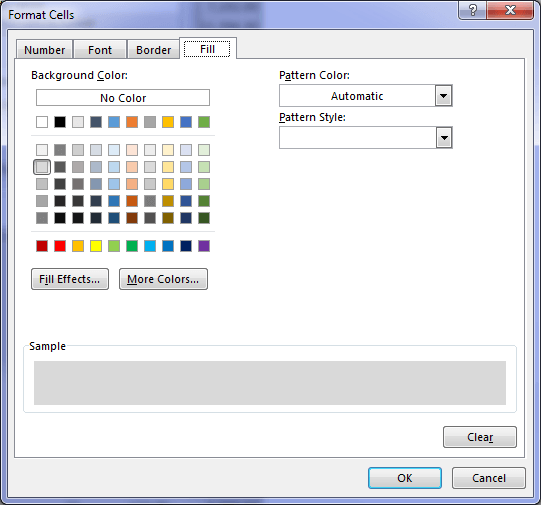
Ok, that’s the formula done, now you can click ‘Format’ to set the fill colour:
More Ideas
You can use the check box technique with other conditional formats. Simply add the AND wrapper like so:
=AND(your conditional format rule, check box cell link = TRUE)
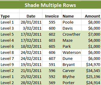
You can also modify the MOD formula to band groups of rows like this:

I want to print Excel specific sheet by choosing on/off sheets name e.g
Sheet1. On.
Sheet2. Off.
Sheet3. On.
Sheet4. On.
Print ok button
Note: All sheets will print except of sheet2.
Hi Naveed, you’d need to write some VBA code to automate this. You might find this dynamic print area technique handy, although it doesn’t do exactly what you want.
Nice tip! Never thought of toggling conditional formatting before – simple but useful!
Cheers, Michael 🙂
While the tip is cool for many applications, there is *SO* much more to tables than banded rows. I routinely use tables for tables in excess of 250,000 rows, though I don’t get crazy with formulas with tables that large, or I shove it into PowerQuery and do the heavy lifting there, then use Excel tables for analysis/filtering/printing.
Yeah, me too, Ed. I’m not saying don’t use tables, I love tables!.
I’m just showing you how to toggle Conditional Formatting on and off and I happened to use the Table style banding as an example 🙂
As for Tables and performance, I’ve seen Tables run into performance issues with as few as 50k rows and also run perfectly well on 500k rows, it really depends on how many columns you have that contain formulas, what type of formulas they are and if you’re running 32-bit Excel or 64-bit Excel. Power Query is absolutely the best place for formula columns and this will allow you to use Tables with much larger data sets.
Mynda
I was curious about the SUBTOTAL function how you prescribe option ‘3’ to “ignore hidden rows.” However, if I manually hid an odd number of rows I would see grey next to grey or white next to white in the banding. By choosing SUBTOTAL option ‘103’ in the formula then the behavior seemed to match your goal.
Hi Don,
If you’re manually hiding rows then yes, 103 ignores these, whereas 3 and 103 ignore rows hidden with filters, which is what I have in my example.
Cheers,
Mynda
Hey Mynda! Where can I find additional background regarding table efficiency: “Unfortunately Excel Tables aren’t efficient with large data sets (over 100k rows)”?
Thanks! And HNY2U2!
Hi Jerry,
I couldn’t find any articles that deal with this specifically, however in my experience if your tables contain lots of formula columns with functions like SUMPRODUCT that operate over arrays and the like, then you’re going to see performance issues. If you’re running 64-bit Excel then you’ll be able to handle bigger tables with more formulas before you see problems, whereas 32-bit Excel users will feel the pain much sooner.
If you have a large table with no formulas and are running 64-bit then you can probably get away with tables containing 500k rows, but a 32-bit user with a table containing lots of VLOOKUP formulas might see issues with only 50k rows. Of course the number of columns will also have an effect.
You might consider shifting the formula calculations to Power Query so the table you bring into the worksheet only contains values, i.e. no formulas.
Mynda
I’ve used conditional formatting to apply banded rows before, but never with an on/off toggle. What a great idea. Now I’m wondering what else I can toggle on/off in a similar way.
Glad you liked it, Mark. Happy formatting 🙂
Dear Mynda,
the use of the SUBTOTAL() function to count the number of VISIBLE nonblank cells from the top row through the current row in a filtered data table is a brilliant idea. To couple this SUBTOTAL() function with a simple MOD() function to distinguish between odd and even numbered rows is an even more clever trick. Thank you so much for sharing this very realistic example with your readers. Now I got another challenge for my prospective students in the spring semester.
Just one “straightforward & trivial” simplification in your excellent conditional formatting formula:
Since the value of the reference cell $I$3 is gonna be nothing but either TRUE or FALSE once linked to the checkbox, there is no need to check its value against “TRUE” once more inside the conditional formatting formula. That is, your conditional formatting formula would still work like a charm if you just rewrite it as follows:
=AND(MOD(SUBTOTAL(3,$A$5:$A5),2),$I$3)
The logical function AND() needs logical statement arguments that result in either TRUE or FALSE. If a cell value is guaranteed to be equal to either TRUE or FALSE anyway, there is no need to construct an equality check with it inside a logical function such as AND() or OR().
Cheers and Happy New Year to Excel Lovers all over the world! – Deniz
Of course, Deniz. Head slap 🙂