It's ok, no zebras get hurt in this process, it's actually all built in to Excel's Conditional Formatting 🙂
Conditional Formatting - Shade Alternate Rows
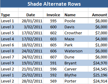
To create this effect we need to create a new rule which uses a formula to determine which cells to format.
Conditional Formatting Using a Formula
- Select the cells you want to shade.
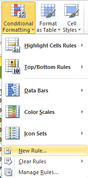
- On the Home tab of ribbon select Conditional Formatting > New Rule
- Select 'Use a formula to determine which cells to format' > enter your formula in the 'Edit the Rule Description' field.
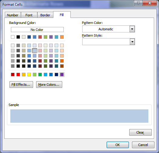
- Click the Format button and from the Format Cells dialog box select the Fill tab > choose your weapon (colour, pattern, fill effect etc.):
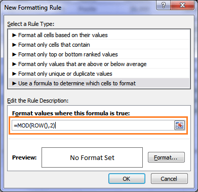
For alternating bands your formula is =MOD(ROW(),2)
Conditional Formatting - Shade multiple rows
You can use a slight variation of the above formula to shade multiple rows like this:
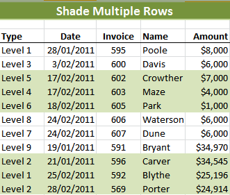
To achieve the above effect you use this formula:
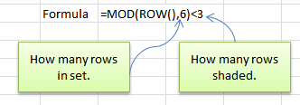
In this formula the 6 states how many rows in the set; 3 shaded 3 not shaded. And the 3 stipulates how many rows are shaded.
You can play around with these numbers to change the number of rows you want shaded and not shaded.
Conditional Formatting - Shade Alternate Rows in a Filtered Table
When your data is filtered you need a slightly different formula for your shaded bands to change as your list is filtered. Otherwise you'll end up with sporadic groups of shaded and unshaded bands.
The formula you want to use is:
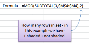
Where cell M4 is the first cell in the header row of your table.
One alternative to the above examples (excluding the Filtered Table) is to simply use Excel's Table tool which automatically inserts shaded bands.
If you liked this trick please share it with your friends on Facebook.

How do I alternate coloring for alternating numbers of rows based on the contents in Column A?
I have a different amount of rows for each inspection report and I want to look at the next number and if it is the same then include it in the current formatting, if it’s different I want to highlight the row in yellow – alternating for every other inspection report number.
inspection numbers date description
86300501 07/14/14 yada, yada, yada
86300501 07/14/14 yada, yada, yada
599000102 08/02/13 more yada, yada, yada
599000102 08/02/13 more yada, yada, yada
599000102 08/02/13 more yada, yada, yada
599000102 08/02/13 more yada, yada, yada
CV4393015 05/21/14
CV4393015 05/21/14
Where the first two rows have yellow highlighting, but the next 4 don’t, then the last two have highlighting. Is that too complex for a single formula? Thanks!
Hi Lory,
It’s not complicated, but you have to use a helper column with a formula to decide if that row should be colored.
Here is a file uploaded on our OneDrive folder.
Catalin
Hi all,
if you do get the error “wrong formula” even when you have entered everything “correct”, please try to replace the “,” with a “;”.
Somehow an US english Excel 2010 (at least in Switzerland) wants to have a “;” instead of a “,” within the MOD command.
Hi Michael,
Thanks for sharing. I know there are many differences with international versions of Excel which most of us with English versions are unaware of.
Cheers,
Mynda.
Hello Mynda,
this is Michael (not Michel) from Switzerland. Did you ever solve the Problem with Michel’s Excel sheet? I am asking as I get here the same error as he does: Wrong formula. I did enter exactly the recommended string. I am using a US Excel 2010.
Hi Michael,
The problem with Michel’s formula was that he still had the double quotes around it. You just enter the formula into the Conditional Format manager like you would into a cell, i.e. without double quotes.
Kind regards,
Mynda.
Thanks for the info on zebra stripes. Does this technique differ in a pivot table? Once you set-up the formula in conditional formatting, do you copy to all the cells in the pivot table that you want to format? Thanks!
Hi Fred,
I would use the Design tools for PivotTables to apply the zebra striping automatically. To locate them simply select any cell in the PivotTable, this should reveal the PivotTable Tools menu on the ribbon. From here you will find the PivotTable styles group where you can choose from a series of predefined stripes or create your own custom style.
Kind regards,
Mynda.
A special thank you for the multiple zebra striping!!
You’re welcome, Noitidart 🙂
Hello
It’s not working..!
We receive always a error (wrong formula)
What can we do?
Hi Michel,
I’m not sure why it’s not working for you. You can send me your file via the help desk and I can take a look at it for you.
Kind regards,
Mynda.
Hi Mynda
Thank you for your support…!
Kind regards from Switzerland
Michel
You’re welcome, Michel 🙂
Thanks for the easy instructions to create Zebra lines in Excel.
You’re welcome, Trudy 🙂