Locating Values in Large Excel Tables

By Harold Graycar XL Numerics Developer of Excel for Customer Service Professionals

The previous post on this topic included a method for finding the cell address for the maximum or minimum number in a table.

Thanks for the correspondence  --  and especially that from Hervé, Saskia and Trevor for the questions about what happens if there are multiple maximum or minimum values.

The previous method sometimes failed where there were multiple maximum or minimum values.

Download Workbook

This version shows a different approach that works reliably under that situation too.

 

1. The ‘index table’ method

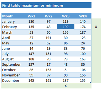
Instead of setting up the reference row and column against the table as shown in the previous model (shown in light green here):

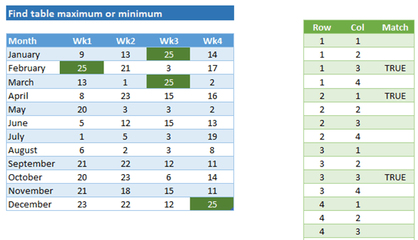
We use a method that works with an ‘index table’ related to the table we are investigating (shown in blue below). And we set up the ‘index table’ (shown in green below) to have one row for each cell in the blue table.

In the index table:

Row 1, Col 1 refers to cell January, Wk1 in the main table

Row 1, Col 2 refers to cell January, Wk2 in the main table

Row 2, Col 3 refers to cell February, Wk3 in the main table

etc.

It may take a few moments to set up the index table, since it needs to have one row for every cell in the table we are investigating (and could be very long if we have a large number of rows and columns in the table we are investigating).

The aim is to get an entry in the index table for each cell in the original table.  In the index table column headed ‘Match’, we do a computation on whether the cell in the original table matches the Maximum (or Minimum if selected).

The formula for each cell in the Match column is:

=IF(INDEX(MyTable,[@Row],[@Col]+1)=Selected,TRUE,"")

This may look a bit complex, but it’s not too difficult if dissected, and it says in English:

Go to the blue table (MyTable). Using the INDEX function, go to the cell given by the Row and Column numbers in the green table.

But wait a minute . . . . how does the ‘+1’ come into the formula?

The first column of MyTable contains the month names, and since we are only interested in the numbers, we add one to the column so we can skip over the month names.  So that means we are considering the Wk1 column to be the first column, the Wk2 column to be the second column, whereas in the Excel table structure, the Month is considered to be the first column and Wk1 is the second column etc.

For each cell in the original table, the index table entry is TRUE if the cell matches the Maximum (or Minimum if selected) and blank if there is no match.

This leaves us with a TRUE value in the index table for every match.  It’s easy to see and verify, too.

 

2. Getting the match information from the index table

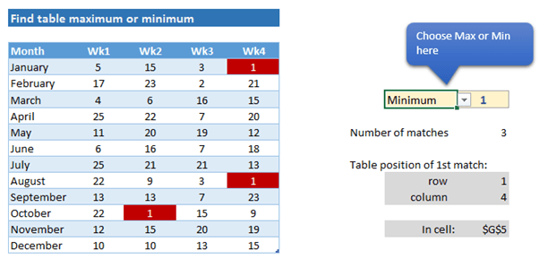
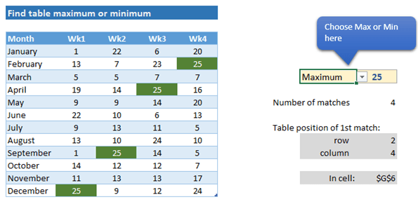
Say this is our result after refreshing the worksheet:

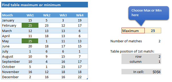
To find the number of matches, we count the number of times the value TRUE appears in the index table column ‘Match’:

=COUNTIF(IndexTable[Match],TRUE)

To find the table position of the first match, the row of the first match in the original table is given by the OFFSET function:

=OFFSET(IndexTable[[#Headers],[Row]],MATCH(TRUE,IndexTable[Match],0),0)

i.e. find the first value of TRUE down the index table (the MATCH function will provide the number of entries down the index table where the first match is located), then use the OFFSET function to count down that same number of rows from the top of the Row column in the index table.

Similarly to finding the row of the first match, the column of the first match in the original table is given by the OFFSET function:

=OFFSET(IndexTable[[#Headers],[Col]],MATCH(TRUE,IndexTable[Match],0),0)

i.e. find the first value of TRUE down the index table, then use the OFFSET function to count down that same number of rows from the top of the Col column in the index table.

Once the row and column of the first match are found, OFFSET can be used again to locate the first matched call in the original table, and to work out its cell address:

=CELL("address",OFFSET(MyTable[[#Headers],[Month]],$L$12,$L$13))

 

3. Some neat conditional formatting

Mynda recently discussed using logical functions to drive conditional formatting, so in this example, I’ve extended that to differentiate between maximum values being found or minimum values being found.

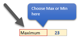
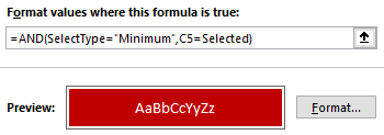
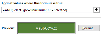
The cell used to denote Maximum or Minimum has the range name ‘SelectType’

So we can set conditional formatting in the original table to be driven by two logical conditions:

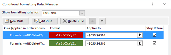
If SelectType is set to Minimum, then paint the minimum cells red:

If SelectType is set to Maximum, then paint the maximum cells green:

So, we’ve covered a more reliable way to locate the row number, column number and cell address largest and smallest numbers – plus some more effective conditional formatting for easily highlighting the locations of those numbers.

There’s a whole lot more on how to use these conditional formatting and formula techniques in the Excel for Customer Service Professionals course.