The GETPIVOTDATA function divides Excel users. You either love it or hate it, but there are good reasons for learning to love it. I wrote about using the GETPIVOTDATA function for regular PivotTables many years ago and hopefully you’re embracing it now. If you’re a Power Pivot user, then you may have found that the GETPIVOTDATA function for Power Pivot, aka the Data Model, works a little differently.
Watch the Video

Download the Workbook
Regular vs Power Pivot GETPIVOTDATA Function
You can easily tell if you’re referencing a regular PivotTable vs a Power Pivot PivotTable because the GETPIVOTDATA function for Power Pivot will have ‘measures’ in the formula arguments, as you can see below:
=GETPIVOTDATA("[Measures].[Average of Order Amount]",$B$9, "[Dates].[MonthName]","[Dates].[MonthName].&[Jan]")
Whereas a regular PivotTable GETPIVOTDATA formula won’t:
=GETPIVOTDATA("Order Amount",$A$4,"Order Date",1,"Years",2009)
Notice the Power Pivot GETPIVOTDATA function also references the table name, field name and item name:
=GETPIVOTDATA("[Measures].[Average of Order Amount]",$B$9,
"[Table Name].[Field Name]","[Table Name].[Field Name].&[Item Name]")
For example:
=GETPIVOTDATA("[Measures].[Average of Order Amount]",$B$9,
"[Dates].[MonthName]","[Dates].[MonthName].&[Jan]")
The Problem with GETPIVOTDATA
GETPIVOTDATA is not relative, meaning if you copy and paste it to another cell it will give you the same results, as you can see below with the formula in cell D11 that simply returns the value for Alberta from cell C11. When copied down to row 23 it returns the same value for Alberta on every row:
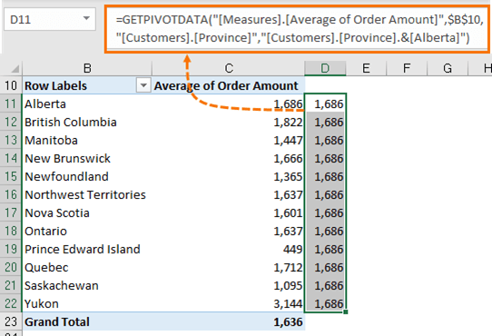
This is because the province, Alberta, is hard-keyed in the formula:
=GETPIVOTDATA("[Measures].[Average of Order Amount]",$B$10,"[Customers].[Province]","[Customers].[Province].&[Alberta]")
Relative GETPIVOTDATA Function for Power Pivot
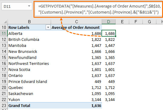
Don’t despair because writing relative Power Pivot GETPIVOTDATA formulas is easy. All we need to do is replace the hard-keyed argument with a reference to the cell containing the province, so that when it’s copied down it picks up the next province.
Using the formula above we replace Alberta with a reference to cell B11, as shown below:
=GETPIVOTDATA("[Measures].[Average of Order Amount]",$B$10,"[Customers].[Province]","[Customers].[Province].&["&B11&"]")
The tricky part is getting the square brackets and double quotes correct so I’ve highlighted the extra characters required in blue font below:
=GETPIVOTDATA("[Measures].[Average of Order Amount]",$B$10,"[Customers].[Province]","[Customers].[Province].&["&B11&"]")
These characters in blue simply concatenate a closing square bracket to the province name. When we copy this formula down, we get relative references that return the Order Amount for the corresponding row:
While the above example handles a single relative reference, we can also make multiple row and column labels relative. In the example PivotTable below, we have both province and month:
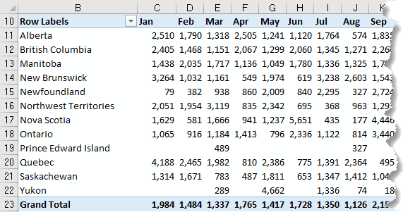
The GETPIVOTDATA formula referencing cell C11 would be:
=GETPIVOTDATA("[Measures].[Average of Order Amount]",$B$9,"[Customers].[Province]", "[Customers].[Province].&[Alberta]","[Dates].[MonthName]","[Dates].[MonthName].&[Jan]")
We can change the province and month values in red font to make the formula relative like so:
=GETPIVOTDATA("[Measures].[Average of Order Amount]",$B$9,"[Customers].[Province]", "[Customers].[Province].&["&B11&"]","[Dates].[MonthName]","[Dates].[MonthName].&["&C10&"]")
Note: In the examples above I am referencing the PivotTable row and column labels, but you can also reference cells on other sheets that contain the province and month names. You just need to ensure the spelling is the same as that found in the PivotTable.
Tip: The GETPIVOTDATA function arguments are:
=GETPIVOTDATA(data_field, pivot_table, field, item,...)
Since we can only replace ‘item’ arguments with cell references, I always let Excel write the GETPIVOTDATA formula first by referencing a PivotTable value cell that I want returned. I then edit the formula and replace the hard-keyed item arguments with cell references.
So, now you have no excuse not to use GETPIVOTDATA. I encourage you to use it because it reduces the risk of formula errors caused by changes to the shape of the PivotTable.
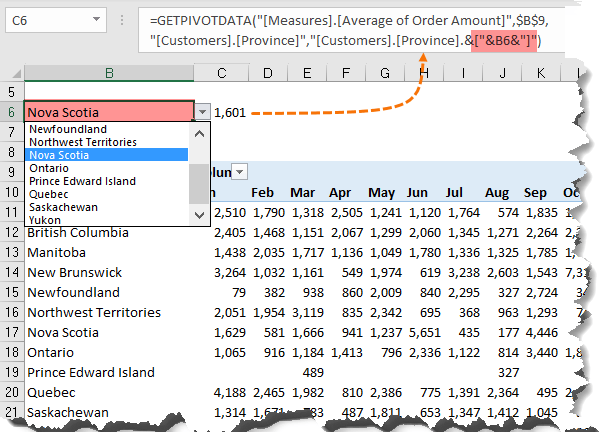
Dynamic GETPIVOTDATA Formulas
The example above deals with copying and pasting GETPIVOTDATA formulas, but sometimes you might want to link it to a drop-down list that allows your user to choose what data they want displayed, as shown below:

I had my getpivotdata working just fine, until I added a subtotal (it doesn’t matter if it’s at the top or bottom of the group) and it turns all getpivotdata formulas into #REF!, even brand new ones if I just type equal and click a value. What is happening that a subtotal breaks the formula?
Thanks
Not sure why that would be, Justin. You’re welcome to post your question on our Excel forum where you can also upload your file and we can help you further.
HI Mynda,
You are one of my favorite youtubers. I have watched many of your videos and they usually solved my problems! Many thanks!
I came across this one when searching for the tips on how to use getpivotdata(). Matching date format in the formula is the biggest takeaway! Now I have a new problem,
In my Power Pivot table, the row field has 2 columns (date and shop), column field is values, and value field has 3 measures (sale1, sale2 and sales3). Depending on the date selected, the number of rows changes. Now my task is to rearrange the pivot table values to make it like the result of unpivot columns in Power Query, i.e., the sale2 and sale3 values will be in the same column and rows labels repeated.
Do you think this is achievable without using VBA?
Thanks in advance!
Hi Tess,
It’s difficult to visualise, but have you tried dragging the sigma (values) item in the column labels well of the PivotTable, down to the row labels well?
If that doesn’t work, post your question on our Excel forum where you can also upload a sample file and we can help you further.
Mynda
Does this allow for a does not equal?
For example, if i want to exclude “Rejected” from my pivot, can i do something like this:
“[Application_Summary].[Admission Status]”,”[Application_Summary].[Admission Status].&[Rejected]”,
to this…
“[Application_Summary].[Admission Status]”,”[Application_Summary].[Admission Status].&&[Rejected]”,
Hi Chris,
Just put the Admission Status field in the Filters area of the PivotTable and set it to exclude Rejected. That way you don’t need to write it into the formula.
Mynda
Thanks a lot! Your video and guidance help me a lot!
Great to hear, Thao!
I tried the formulae structure like you outlined but I get REF ERROR.
Power Pivot Table
=GETPIVOTDATA(“[Measures].[Sum of Budgeted Sales]”,$D$3,”[Budget].[CalendarYear]”,”[Budget].[CalendarYear].&[2.001E3]”)
=GETPIVOTDATA(“[Measures].[Sum of Budgeted Sales]”,$D$3,”[Budget].[CalendarYear]”,”[Budget].[CalendarYear].&[“&G4&”]”)
G$ value from date column
Can figure out where I went wrong
Hi Gerry,
I suspect the value in cell G4 is not in the format 2.001E3
Mynda
Hi
I tried to use the modification but its still giving me an error, not sure if im doing something wrong. the original and modified formula is as below:
original:
=GETPIVOTDATA(“[Measures].[Distinct Count of Name]”,Output_PVT!$A$156,”[Table1 date Name].[date]”,”[Table1 date Name].[date].&[Aug-17]”,”[Table1 date Name].[P value]”,”[Table1 date Name].[P value].&[]”)
modified:
=GETPIVOTDATA(“[Measures].[Distinct Count of Name]”,Output_PVT!$A$156,”[Table1 date Name].[date]”,”[Table1 date Name].[date].&[“&I1&”]”,”[Table1 date Name].[P value]”,”[Table1 date Name].[P value].&[“&O9&”]”)
Hi Mohammad,
The original formula implies the P value is blank, so if you’re now trying to insert a P value from cell O9, perhaps that’s the problem. It’s impossible to say for sure without seeing your file. If you’re still stuck please post your question on our Excel forum where you can also upload a sample file and we can help you further.
Mynda
Thank you, this was extremely helpful.
Great to hear!
Thank you for this awesome post it was really helpful and saved my day. I cleared most of the stuff following the details above but I am stuck at one pont. It will be really helpful if you can guide me.
Cell A2 has date which is coming from a link to another cell
=IFERROR(IF(Pivots!BE6=”Grand Total”,””,IF(Pivots!BE6=0,””,’Data Model’!AX4)),””)
Cell B1 has hard coded time as (0,1,2,3…… 23)
In Cell B2 I am trying to run the GETPIVOTDATA and it is showing the result, but as soon as I make it ref to cell A2 to get the date it is throwing an error.
=GETPIVOTDATA(“[Measures].[Count of Incident #]”,’Data Model’!$AZ$3,”[Range 1].[Time]”,”[Range 1].[Time].&[“&B$1&”]”,”[Range 1].[Date]”,”[Range 1].[Date].&[“&VALUE(A2)&”]”)
Please help.
PS. Will not be able to share the file as has office data.
Hi Rajiv,
You need to look at the format of the date in the PivotTable that you want to replace with a cell reference and ensure the cell A2 uses the exact same format. And when I say format, I mean the underlying value in the cell must match the way it is stored in the PivotTable. If you build the GETPIVOTDATA formula using your mouse you will be able to see what Excel is expecting in the Time component of the formula. I hope that helps.
Mynda
Thank you Mynda for the quick guide. Yes it does and I did try doing that earlier but the issue was still there. I have created a sample file but not able to find a place to upload the same ;(
as was unable to find the upload option sharing the drive link to the file. Hope it helps
https://drive.google.com/file/d/1NIXYx1qahVRQhEQ6-Aa_6-DBqF93dLe8/view?usp=sharing
Hi Rajiv,
Thanks for sharing your file. If you enter the GETPIVOTDATA formula by selecting the cell B5 on Sheet3 you can see this formula is returned:
=GETPIVOTDATA("[Measures].[Count of Incident #]",Sheet3!$A$3,"[Range].[Date]","[Range].[Date].&[2020-09-01T00:00:00]","[Range].[Time]","[Range].[Time].&[1]")The problem in your formula is caused by the date reference. You can see above the date is [2020-09-01T00:00:00] i.e. including the time element, but the dates in column A of Sheet2 are only the date portion.
Replace your formula in cell C2 of Sheet2 with this formula:
=GETPIVOTDATA("[Measures].[Count of Incident #]",Sheet3!$A$3,"[Range].[Date]","[Range].[Date].&["&TEXT($A2,"yyyy-mm-dd")&"T00:00:00]","[Range].[Time]","[Range].[Time].&["&C$1&"]")Mynda
Thank you Thank You Thank You Mynda… You are a real life saver 🙂
My pleasure, Rajiv!
Hi there,
Has the referencing convention changed for relative GETPIVOTDATA in excel office 365? I use exactly as instructed above, but keep getting #REF error.
Excel formual is: =GETPIVOTDATA(“[Measures].[GRPs]”,$A$7,”[F_GRPTracking].[Brand]”,”[F_GRPTracking].[Brand].&[OUTSURANCE]”)
I changed the last square bracket hard code to: =GETPIVOTDATA(“[Measures].[GRPs]”,$A$7,”[F_GRPTracking].[Brand]”,”[F_GRPTracking].[Brand].&[“&A13&”]”).
If I input another set of ” after the & as suggested by Catalin, I get the “excel thinks this is a formula” error.
thanks
Tracy.
Hi Tracy,
Can you select this section of the formula: “[F_GRPTracking].[Brand].&[“&A13&”]” (including all double quotes) in the formula bar, then press F9 Key?
You should see in formula bar the result of that concatenation, should be like: “[F_GRPTracking].[Brand].&[OUTSURANCE]”
Make sure the value you have in A13 is exactly the same, (no invisible chars like spaces for example), is visible in the pivot, the ref error is returned if that item is not visible.
Hi, I’m sure I’ve done this before and it worked but it doesn’t anymore – has something changed? Or am I missing something? The formula provided by Excel is:
=GETPIVOTDATA(“[Measures].[Sum of Employees]”,$A$79,”[Employees per month].[Month End]”,”[Employees per month].[Month End].&[2019-02-28T00:00:00]”)
I want to make the last set of square brackets dynamic so I changed it to this:
=GETPIVOTDATA(“[Measures].[Sum of Employees]”,$A$79,”[Employees per month].[Month End]”,”[Employees per month].[Month End].&[“&B80&”]”)
But I get a #REF error. In the pivot table, row 81 is the total row, row 80 is the header row. The pivot table has no rows in between. Is this the problem?
Is the formula correct? I don’t see a double quote:
[Month End].& “ [“&B80&”]”)
Make sure you test it on a pivot that has data, not an empty PT.
Cheers,
Catalin
What are [Customers] and [Dates] referring to in these examples? They are neither visible nor explicit. I am trying to extract Distinct Count of Months where multiple criteria are met. Some are 3 months, some are all 12, but trying to figure out how to assemble the references is not articulated on two dozen sites I have already tried to get this answer from.
Hi Nicholas,
Power Pivot GETPIVOTDATA formulas reference the table, field and item e.g. =GETPIVOTDATA(“[Measures].[Average of Order Amount]”,$B$10,”[Table].[Field].&[Item]”)
[Customers] and [Dates] are referring to tables with those names. If you’re trying to do a distinct count then you don’t need GETPIVOTDATA, you can simply use Distinct Count in Power Pivot.
Mynda
My data is a connection only w/ data model enabled and my dates when using a pivot table associated w/ GetPivotdata is giving me #REF! errors. However, if I use “Close & Load” which directly uploads the data into a table within Excel the GetPivotData formula works correctly as you outline above ([“&B11&”]”,”[Dates].[MonthName]”,”[Dates].[MonthName].&[“&C10&”]”)). I need to change the direct identifiers within the GetPivotData formula associated w/ my pivot table to a cell reference (as shown above) within a report due to the massive file size of the raw data but haven’t found the resolution as of yet. I used your instructions shown above within the GetPivotData formula for all references and they have worked except for the date reference. I’ve made sure the Data Model and Power Query have the column as a date, check Excel (pivot table) and it is also identified as a short date, but each time I use the same instructions as shown above on your site I only get #REF! error.
Hi Mark,
I usually reference the value cell and allow GETPIVOTDATA to write the formula so I can see the exact structure of the date fields it’s looking for. Usually the month is a text field, as opposed to a date formatted as mmm. If you’re still stuck, please post your question on our Excel forum where you can share a sample Excel file or screenshots.
Mynda
How do we use the VBA method GetPivotData when using the Data Model?
Hi Nicolas,
Have you read this?
https://docs.microsoft.com/en-us/office/vba/api/excel.pivottable.getpivotdata
If you have a specific question or problem you can post it on our forum.
Regards
Phil
Thank you. You have no idea how long I looked for the answer to this! I have a grouped months field as columns and a grouped year field as rows. I wanted to have a simple table on another sheet which referenced this data. All other “help” on the internet didn’t come close to solving this problem, but you did.
What a relief!
So glad we could help, Tobias 🙂
Great info, thanks! I am struggling with making a formula have a dynamic “year” reference. I pull data to an excel sheet from a power pivot, and have the nation change dynamically, but the year does not. Any thoughts? This is what I have so far- =GETPIVOTDATA(“[Measures].[Sum of IMPORTS_QTY]”,Data!$A$5,”[NATION_ANNUAL].[YEAR]”,”[NATION_ANNUAL].[YEAR].&[1.99E3]”,”[NATIONS].[LT_KSD_NATION_NAME]”,”[NATIONS].[LT_KSD_NATION_NAME].&[“&$B15&”]”) . The start year is 1990, and I do not understand what the 1.99E3 does. Thank you!
Hi Mike,
1.99E3 is equal to 1.99*10^3=1990
Thanks Catalin! I am now more smarterly. What I cannot figure out is how to make that dynamic, so I can replace 1.99E3 with a cell reference and have it not throw the #REF error. I hit two different tables in an Access db and join them in a power pivot, then use that as a data source. As a Band-Aid I tried writing the full query in Access and hitting THAT as a data source, and then this works: =GETPIVOTDATA(“IMPORTS_QTY”,Data2!$A$5,”LT_KSD_NATION_NAME”,$B18,”YEAR”,C$1) where B is Nations and C is Years. I am trying to discover a way to edit the initial example to dynamically change the year as well as the nation to roll out to several other projects. Any tips are tremendously appreciated!
Hi Mike,
Not sure why it takes the year in scientific format, but you have to format the cell in the same format, if that’s what the formula needs.
I had a similar issue that I resolved as follows…
In my case, the underlying data model was created through PowerPivot. Through PowerPivot, you can see the formatting type when you select the column in question and then review “Home > Formatting > Data Type” within the PowerPivot ribbon. Most likely, the formatting is set up a decimal number. If you change the formatting to whole number, you should now be able to reference GetPivotData as a whole number!
Brilliant. Thanks 🙂