Show Values as Percentage of Another PivotTable Column Total

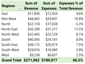
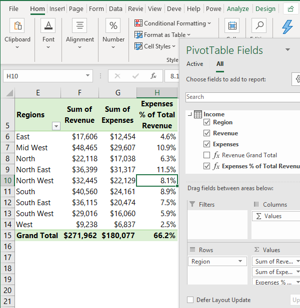
Occasionally you may want to show values as percentage of another PivotTable column total. For example, below we want to find what percentage the expenses for each region are of the total revenue:

Unfortunately, you can’t do this with regular PivotTable calculated fields or PivotTable calculated items.

However, we can with Power Pivot*, aka the Data Model. All we need to do is write a DAX measure, but don’t worry, it’s super easy.

*Note: Not all versions of Excel come with Power Pivot. Click here to check if your version of Excel has Power Pivot.

Power Pivot Show Values as % of Another PivotTable Column Total

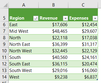
Below is the source data I’ve loaded into Power Pivot. It’s just a small sample, in reality you’d be aggregating hundreds, thousands or even millions of rows of data. Yes, Power Pivot can handle millions of rows of data.

Load Data to Power Pivot

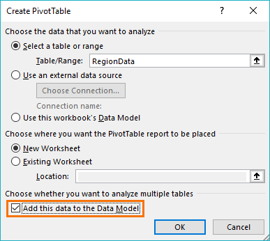
In Excel 2013 onward, you can load data from an Excel table into Power Pivot by checking the ‘Add this data to the Data Model’ box when inserting a PivotTable.

In Excel 2010 you can click on the ‘Add to Data Model’ icon on the Power Pivot tab:

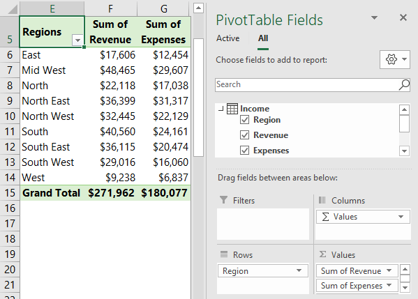
Build the PivotTable

Build the PivotTable bringing the Revenue and Expenses fields in to the Values area as you normally would.

Write the DAX Measures

Now all we have left is to create the measures.

We need a measure that calculates the Total Revenue and then one to calculate the Expenses as a percentage of total Revenue. That said, you could write it all in one measure, but it's common practice to create the building blocks separately so they can be re-used in multiple measures.

We’ll create the total Revenue measure first since we need to reference this in the percentage calculation.

On the Power Pivot tab of the ribbon > Measures > New Measure*

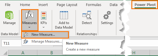
*In Excel 2013 Measures were called ‘Calculated Fields’.

This opens the New Measure dialog box where you can (1) give your measure a name, I’ll call it ‘Revenue Grand Total’, (2) enter the DAX formula, (3) set the formatting:

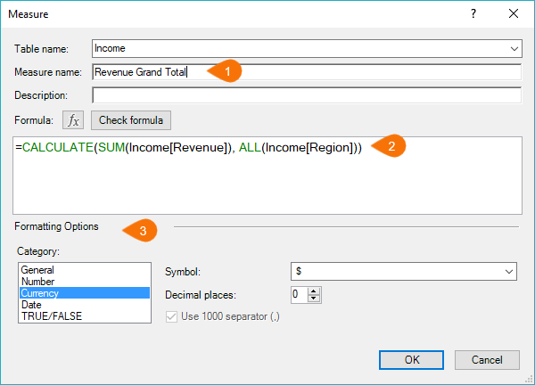
The DAX formula:

=CALCULATE(SUM(Income[Revenue]), ALL(Income[Region]))

In English it reads:

CALCULATE the SUM of ALL income irrespective of any Region filters, or row and column context.

Notice the formula uses Structured References, just like an Excel Table. E.g. SUM(Income[Revenue])

While we don’t need this measure in the PivotTable, if we were to insert it, as you see below, the Total Revenue is entered in every cell:

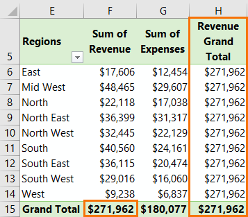
We can then use this measure as the denominator in our percentage calculation.

Let’s do that. I’ll create my Value as percentage of Another Column Total, which is Expenses / Revenue Grand Total. The DAX formula is:

=DIVIDE(SUM(Income[Expenses]), [Revenue Grand Total])

The DIVIDE function handles #DIV/0! Errors. In English it simply reads, DIVIDE the SUM of Expenses by the Revenue Grand Total.

Notice the formula refers to the first measure; ‘Revenue Grand Total’.

Now I can insert that measure in the Value field of my PivotTable like so (note: I removed the ‘Revenue Grand Total’ measure because I don’t want it in my PivotTable report):

So, you see DAX formulas aren’t that scary.

Download the Workbook

Note: This workbook is compatible with Excel 2013 onward.

Power Pivot Data Sources

In this example the data was in the Excel file, but you can also get data from tons of external sources or load direct from Power Query to the Power Pivot Data Model. Unfortunately, I haven’t got time to cover them all here.

If you’d like to learn Power Pivot, please consider my Power Pivot Course.