Extracting Text Strings Using Excel’s Text to Columns

The Easy Way

In this example I’m going to show you how you can extract the domain name from a URL in Excel.

For example, taking the list of URL’s below we want the part in between the http:// or https://, and the next forward slash.

So the domain for the first URL below is www.ikea.com

There are two approaches:

1. The really complicated, banging head on desk, formula method or
2. The click a few buttons Text to columns method.

I don’t know why but most people choose the formula option. Probably because they don’t know Text to Columns exists.

Don’t get me wrong. Formulas have their place (and I’ll cover them next week), but unless you’re setting up a template that you’re going to use over and over again, Text to Columns is your best friend.

Text to Columns

You’ll find the Text to Columns tool on the Data tab of the ribbon in the Data Tools section:

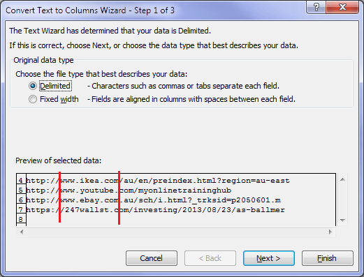
Clicking on the Text to Columns icon opens the Wizard in step 1 of 3:

Here you have to choose the file type that describes your data.

The rules are simple:

If you can draw a straight vertical line (that represents a column), between the data you want to separate, then you choose Fixed Width. If you can’t, then you need to choose Delimited.

You can see in the image below I’ve put a red line where I want the text separated, but the last row is going to leave a forward slash at the front of my domain.

Not to mention, the domains aren’t the same length so I can’t draw vertical lines after the .com/ part either.

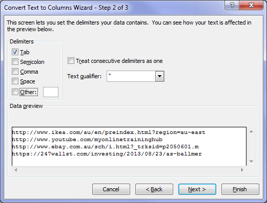
So, in this case I need to choose the Delimited data type. Pressing ‘Next’ brings me to step 2 of the Wizard:

Here I can choose the delimiter I want to use to separate my data. Common delimiters are Tab, Semicolon, Comma (think .csv files) or Space, but I can also stipulate another delimiter that occurs in my data.

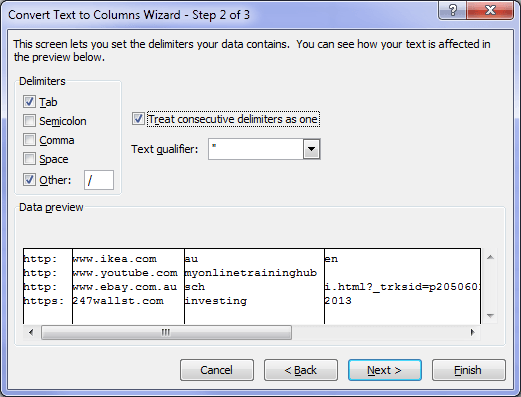
Since I want the data after the http:// I’m going to use the forward slash as my delimiter (also check the ‘Treat consecutive delimiters as one’ so that the // after the http: is not given its own column).

As soon as I enter the slash in the ‘Other’ field the Wizard gives me a preview of how my data will be separated.

Each set of data between a / is separated into its own column as indicated by the vertical lines in the Data preview section below:

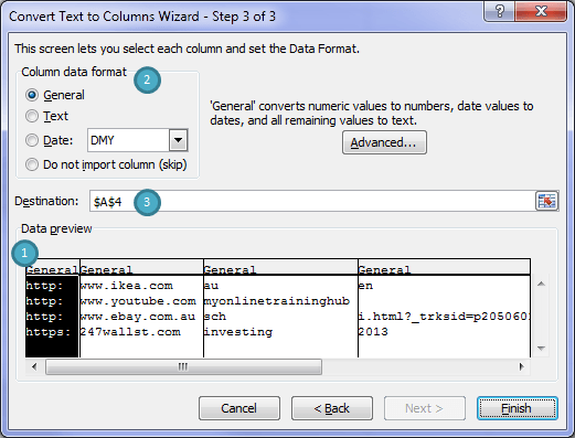
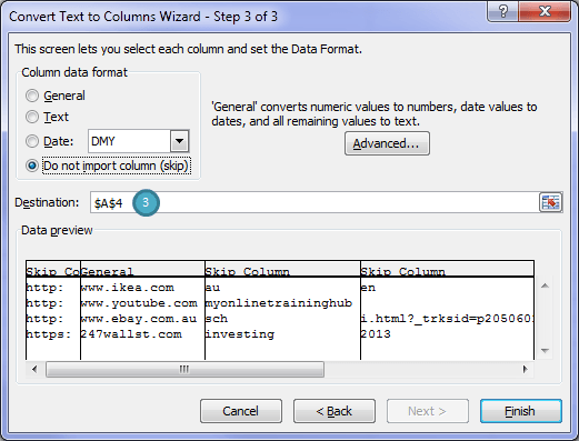
In the next step I can choose which columns I want to keep (1) and in what format (2), and where to place the extracted data (3):

I only want to keep the column containing the domain so I’m going to select each column I don’t want by clicking in the column to select it (1), then in the ‘Column data format’ section (2) I’m going to select ‘Do not import column (skip)’.

You can see in the image below all of the column headers now read ‘Skip Column’ except the column containing the domain which I’m going to keep.

Lastly I can choose the cell Destination for the domain names (3).

Tip: if you want to retain the original URL make sure you change the destination cell (3) to a cell in an empty column, otherwise it will replace your original data.

Finished Product

Here we have our domain names in under a minute, and without bruising to your head. 🙂

Tip: Sometimes you need to run your data through Text to Columns in stages, extracting one part of the data in the first pass, then the next part, and so on. It all depends on the delimiters in your data.

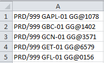
Let’s take the data below as an example:

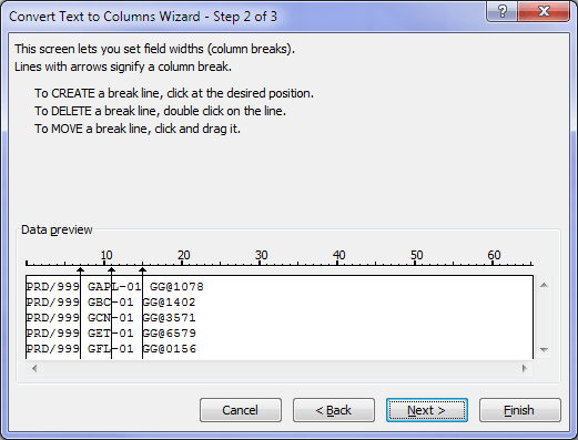
It’s almost in the right format to just use the Fixed Width format in step 1 of the Wizard, but we can see (image below) when I choose this option that it’s not quite right because the first row has 1 character too many in the second column:

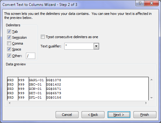
That’s ok, I can use the Delimiter method like this:

See in the image above how I’ve selected several delimiters based on what is present in my text.

I’ll need to run it through the Text to Columns twice though because I also want to separate the 01 from the preceding text and I can only choose one ‘Other’ delimiter at a time.

Other Uses for Text to Columns

Another great use for Text to Columns is fixing dates formatted as text.

Next week I’ll step you through the formula method. Don’t worry there’s no need to tape bubble wrap to your head in anticipation of banging your head on the desk.

I’m going to show you an easy way to build complex MID formulas without the usual frustration.