If you’ve worked with dynamic array formulas*, you’ll have noticed that they’re able to spill the results to multiple cells. For example, in the image below we can see the UNIQUE function has spilled the results to cells G3:G6 which are highlighted with a blue border:
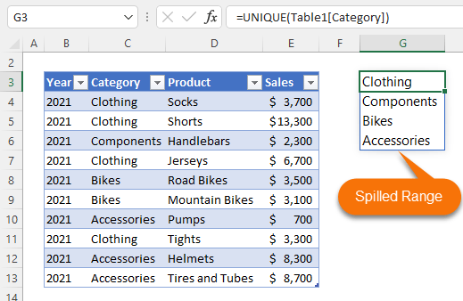
With the hash sign in Excel formulas we can easily reference that spilled array by appending it to the first cell reference for the array like so:
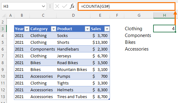
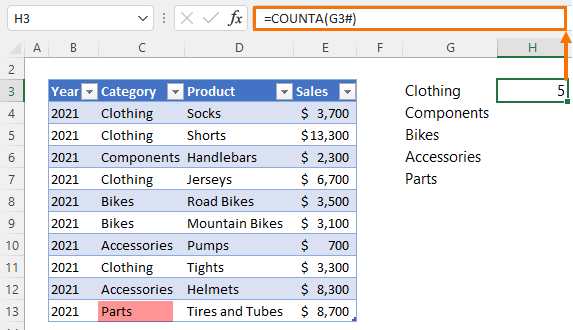
This is easier to write, but more importantly it’s dynamic. For example, if the category in cell C13 is changed to ‘Parts’, we now have 5 different categories and without having to update any formulas, they automatically update:
Fun fact, the official name for the hash sign is Octothorpe (thanks to Roger Govier for that fun fact). In Excel it's referred to as the Spill Operator as it enables us to reference spilled arrays.
*Note: Dynamic array formulas are available in Excel 2021 and Microsoft 365.
Watch the Video

Download Workbook
Enter your email address below to download the sample workbook.
Excel # Spill Operator Examples
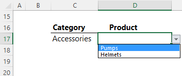
Let’s say I want to create dependent data validation lists for the Category and Products like this:
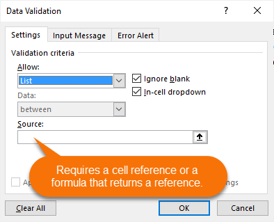
The data validation list requires a reference to cells, or a formula that returns a cell reference (remember dynamic array formulas return an array):
Therefore, I can’t use a dynamic array formula directly inside the data validation dialog box to return the list. Instead, I need a table containing the different products in lists by category. I can use TRANSPOSE with UNIQUE for the column headers containing the categories, and FILTER for the product lists:
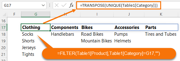
Note: the filter formula in cell G18 is copied to columns H:N to allow for growth in the number of categories.
Now that I have the table for each category and its products, I can reference this in my data validation lists.
Referencing Spilled Arrays in Data Validation
Because the table above contains spilled arrays, I can use the # operator to reference them ensuring I always pick up any changes to the table.
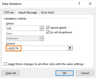
Category Data Validation List: To set up the data validation list for the Categories I can reference cell G17# in the data validation list dialog box:
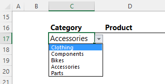
If I add any more categories to the table, the data validation list will automatically include them.
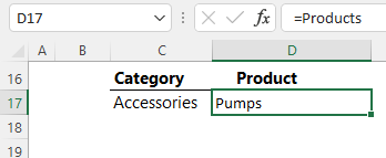
I’ve inserted the data validation list in cell C17:
Now I need the dependent data validation list for the Products.
Referencing Spilled Arrays with Dynamic Named Ranges
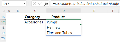
Product Data Validation List: The dependent data validation list needs to lookup the category selected in cell C17 and return the relevant list of products. I’ll use the XLOOKUP function to return the reference to the product list.
The trick here is to reference the first row of the FILTER results in row 18 and append the spill operator to the end of the formula:
=XLOOKUP(C17,$G$17:$N$17,$G$18:$N$18)#
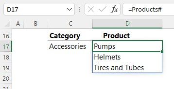
I can use this formula in a cell, and it spills the results:
Or, because XLOOKUP returns a reference, I can alternatively use this formula in my data validation list source:
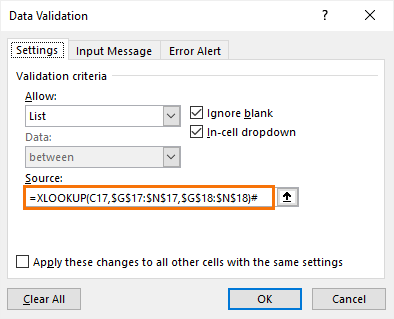
This returns the products that spill from the FILTER formulas in row 18.
Note: You might be wondering why in the XLOOKUP formula I haven’t referenced the spilled array in G17 like this:
=XLOOKUP(C17,$G$17#,$G$18:$N$18)#
And that’s because if the size of the list of categories changes the return array will be the wrong size and the formula will return an error.
Instead, I’m referencing G17:N17 which also allows me to lookup out to column N allowing for growth in the list of categories. Obviously, you can extend this further than column N to allow for even more growth.
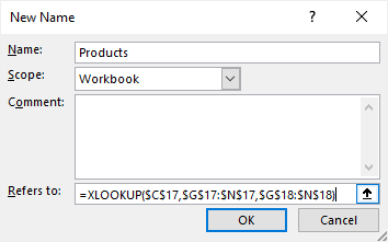
Cool Trick with Defined Names
Another way we can use the # spill operator is by appending it to a defined name. For example, we can define a name for the Products using an XLOOKUP formula with or without the #. I’ll define it without the #:
If we look at this name in a formula you can see it returns the first item in the spilled array:
But when we append the spill operator to the name, we get the spilled array:
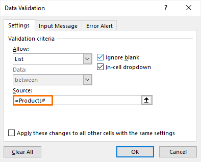
Therefore, in the data validation list we can also access the spilled arrays by appending # to the defined name:
The purpose of this tutorial is to illustrate the different ways we can use the spill operator. There’s no benefits either way, it’s really what you’re most comfortable working with.
More Dynamic Arrays
If you'd like to get up to speed with dynamic arrays, please consider my Advanced Formulas Course.

As always, thank you for the awesome tutorial! I thought it would be cool if the formula were to be enhanced to make it a little more dynamic.
You addressed why this formula: =XLOOKUP(C17,G17:N17,G18:N18)# used the G17:N17 lookup range as opposed to using G17 with the spill operator, like in this formula: =XLOOKUP(C17,G17#,G18:N18)#. Since the issue is with the return array, I tried to construct that by counting how many items are in the spilled array and then using the ADDRESS function for the last item in the spilled array nested in an INDIRECT to return the range to the XLOOKUP, like so: =XLOOKUP(C17,G17#,INDIRECT(“G18:”&ADDRESS(18,6+COUNTA(G17#),,1)))#. Then I realized it could be tidied up a bit with OFFSET, like so: =XLOOKUP(C17,G17#,OFFSET(G18,0,0,,COUNTA(G17#)))#.
Certainly, the solution you provided is the simplest. But I am wondering if you see any other downsides to implementing one of these next-level formulas? … I know some people prefer to avoid INDIRECT due to its volatility.
Great ideas, John. Someone else also shared the OFFSET solution on my YouTube channel. I prefer that to INDIRECT although they’re both volatile, which is fine as long as there aren’t loads of them in your file.