Oh, how I wish I’d had the fortune of the new Excel XLOOKUP function back in my accounting days.
The first powerful function I learnt was VLOOKUP. It gave me a sense of power and cemented my love of Excel.
XLOOKUP is everything VLOOKUP is and much more.
- XLOOKUP can look up to the left
- XLOOKUP won’t break if columns are inserted or deleted in the lookup array
- XLOOKUP can find the last occurrence of a value
- XLOOKUP defaults to an exact match, so new users won’t accidentally return erroneous data
- XLOOKUP can return a range of cells or a single cell, just like INDEX
- XLOOKUP allows you to specify an alternate value if the lookup value is not found. No more need for IFERROR.
Table of Contents
XLOOKUP Function SyntaxDownload Example File
XLOOKUP Function Video
XLOOKUP Formula Examples:
1. Simple XLOOKUP Formula
2. XLOOKUP Function does HLOOKUP
3. XLOOKUP Function does INDEX & MATCH
4. XLOOKUP Formula Returns Multiple Columns
5. XLOOKUP Dynamic Range
6. XLOOKUP Function Error Handling
7. XLOOKUP Last Value
8. XLOOKUP Left
9. XLOOKUP Function Wildcards
10. XLOOKUP Function Approximate Match
XLOOKUP Function Syntax
With all this new functionality comes some more arguments, so let’s look at the syntax:
=XLOOKUP( lookup_value, lookup_array, return_array, [if_not_found], [match_mode], [search_mode])
Don’t be put off by the number of arguments in this function because most of the time you’ll only use the first three and it is still way easier than VLOOKUP.
| Argument | Description |
| lookup_value | The value you want to find, or cell containing the item you want to find |
| lookup_array | The cell range or array you want to search |
| return_array | The cell range or array containing the value you want returned |
| [if_not_found] | Optional - the text you want returned in the event a match isn't found. If omitted an error will be returned |
| [match_mode] | Optional - Defaults to 0 for exact match 
|
| [search_mode] |
Optional - Defaults to 1 searching first to last  |
| Options 2 and -2 require the lookup_array to be sorted in ascending or descending order respectively*. |
Notes:
*Binary search does not result in faster calculations now that Microsoft have optimised the lookup algorithms.
The lookup_array and return_array must be the same size, otherwise the #VALUE! error will be returned.
If XLOOKUP references another workbook the #REF! error will be returned if the external workbook is closed.
The XLOOKUP function is currently only available to Office 365 users on the Insider channel. If you can’t wait, you can try it out in Excel Online.
Download Workbook
Enter your email address below to download the sample workbook.

Watch the Video

Excel XLOOKUP Function Examples
XLOOKUP is a versatile function and will allow the average Excel user to conquer tasks that previously required multiple functions.
1. Simple XLOOKUP Formula
In its most basic form XLOOKUP searches a range of cells and returns an item corresponding to the first match it finds.
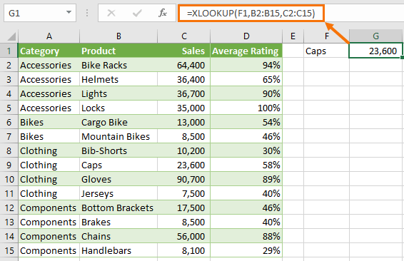
The lookup_array doesn’t need to be sorted because XLOOKUP will return an exact match by default.
In English the formula above reads, lookup the value in cell F1, which is Caps, in cells B2:B15 and return the value on the corresponding row in cells C2:C15. If you don’t find an exact match, return an error. This last part is the default behaviour because I didn’t provide a value in the if_not_found argument.
One benefit of this formula over the VLOOKUP equivalent =VLOOKUP(F1,B2:C15,2,0) is that it won’t break if a column is inserted between columns B and C.
2. XLOOKUP Function does HLOOKUP
Not only does XLOOKUP replace VLOOKUP, but it can also perform HLOOKUPs:
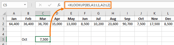
Important: A vertical lookup_array must contain the same number of rows as the return_array and a horizontal lookup_array, as in this example, must contain the same number of columns as the return_array.
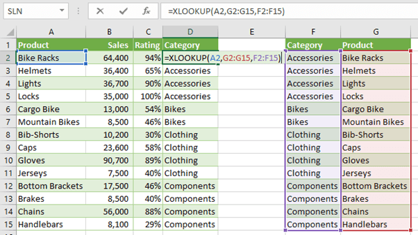
3. XLOOKUP Function does INDEX & MATCH
The formula below crafted by MrExcel himself (aka Bill Jelen), reads: look up Feb in cells A2:A13 and return the value in the range that corresponds with the column Clothing is in.
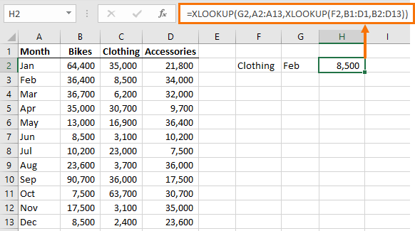
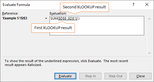
If you look at the Evaluate Formula dialog box below you can see the second XLOOKUP returns a range:
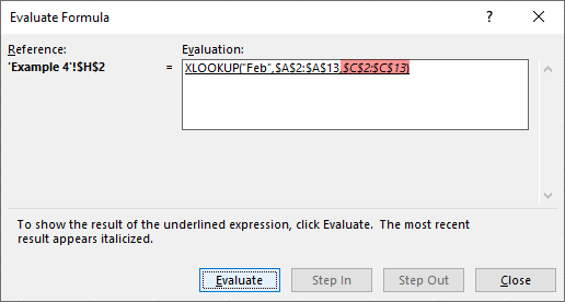
The fact that XLOOKUP returns a range is what enables us to nest it in the return_array argument.
That said, it’s probably easier to understand an equivalent INDEX & MATCH formula:
=INDEX(B2:D13,MATCH(G2,A2:A13,0),MATCH(F2,B1:D1,0))
Or even the new XMATCH* function which is shorter because it defaults to an exact match meaning the third argument is not required:
=INDEX(B2:D13,XMATCH(G2,A2:A13),XMATCH(F2,B1:D1))
*XMATCH is another new function available to Office 365 users on the Insider channel. For the most part it’s the same as the MATCH function except it defaults to an exact match.
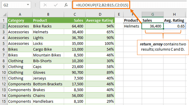
4. XLOOKUP Formula Returns Multiple Columns
In the formula below the return_array argument is columns C and D. With Office 365 XLOOKUP will return multiple values as dynamic arrays allow XLOOKUP to spill the results.
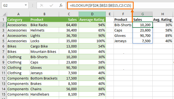
Note: Currently the Excel calc engine can only support spilling XLOOKUP in one direction, either across columns, as in the example above, or down rows as in the example below:
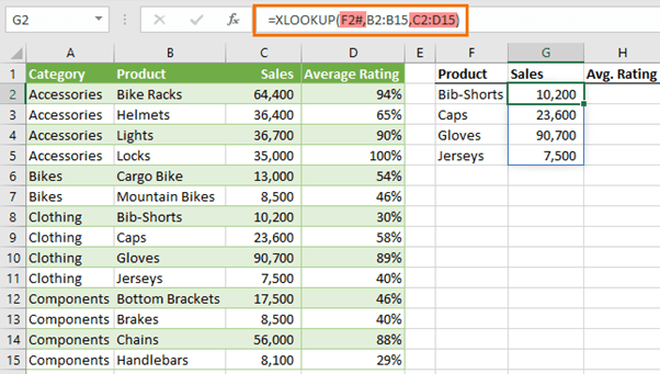
If your XLOOKUP formula results in two spilled ranges, as in the example below, only the first range will spill:
You can return non-contiguous columns with CHOOSE in the return_array:
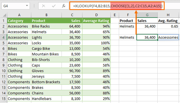
Thanks to fellow MVP, Wyn Hopkins for the CHOOSE function idea.
5. XLOOKUP Dynamic Range
Now that we know XLOOKUP can return a range, we can use it to return a dynamic range, which you can name. No more need for OFFSET or INDEX & MATCH to create dynamic named ranges.
In the example below I want to sum the sales values from the start date (G3) to the end date (H3).
Note: My dates are dd/mm/yyyy.
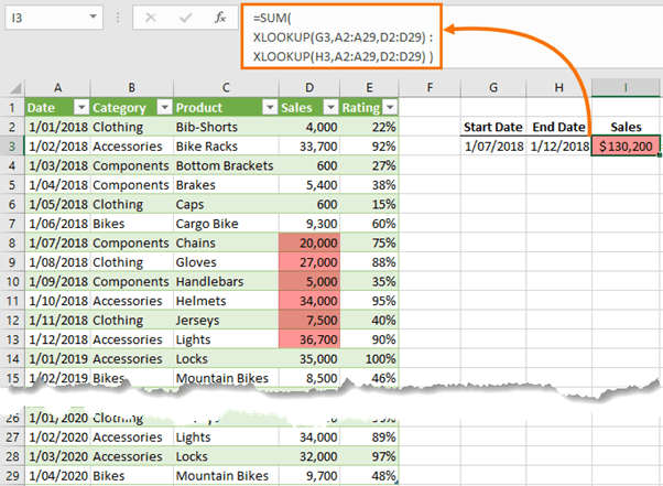
We use two XLOOKUP formulas either side of the colon range operator. The first XLOOKUP formula returns the first cell in the range and the second XLOOKUP formula returns the last cell in the range:
=SUM( XLOOKUP(G3,A2:A29,D2:D29) : XLOOKUP(H3,A2:A29,D2:D29) )
You can see how it evaluates in the Evaluate Formula dialog box below:
By now you’re probably thinking that XLOOKUP is a function killer. It has already done away with VLOOKUP, HLOOKUP, INDEX & MATCH and OFFSET, but wait, there’s more! So far, we’ve only used the first 3 arguments. There are still 3 optional arguments to explore.
6. XLOOKUP Function Error Handling
Back in the early days of VLOOKUP we used IF(ISNA(VLOOKUP… to handle errors. Then came IFERROR which made life simpler and more efficient for Excel. But with XLOOKUP we don’t need any extra functions to handle errors because the fourth argument, if_not_found, allows us to specify a value to be returned in the event XLOOKUP doesn’t find a match.
In the example below I’ve entered the text ‘Not Found’ in the if_not_found argument. Alternatively you can enter numbers, another formula, an array or cell reference.
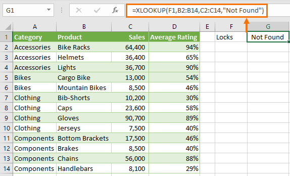
Note: If you omit the if_not_found argument and a match cannot be found, XLOOKUP will return #N/A.
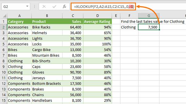
7. XLOOKUP Last Value
By default, XLOOKUP searches first to last, which is search_mode 1. Using -1 in the search_mode argument tells XLOOKUP to search from the bottom up, thus finding the last matching value. The image below shows XLOOKUP returning the last Sales value for Clothing:
You may have noticed that with 2 or -2 we can also perform binary searches where our lists are sorted:
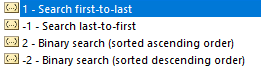
In earlier versions of Excel, binary searches evaluated more quickly, but according to Microsoft in Office 365 this is no longer the case. As a result, there is no significant benefit to using the binary search options and in fact it’s easier to use 1 or -1 search modes because they don’t require the table to be sorted.
8. XLOOKUP Left
One of the limitations of VLOOKUP is the inability to return values to the left of the lookup column. XLOOKUP isn’t hindered by that limitation, as you can see below:
If you don’t have the XLOOKUP function you can use INDEX & MATCH or the workaround with CHOOSE to trick VLOOKUP into looking up to the left.
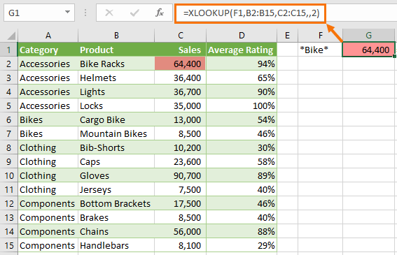
9. XLOOKUP Function Wildcards
VLOOKUP supports wildcards for partial matches by default, which meant looking up words that contained a wildcard like an asterisk e.g. *Alpha, would require the wildcard character to be prefixed by the tilde e.g.:
=VLOOKUP( "~*Alpha", B2:C15, 2, 0)
XLOOKUP only supports wildcards if you specify 2 in the match_mode argument and therefore you don’t need to prefix the wildcard with the tilde:
Note: Wildcards cannot be used in binary search mode.
10. XLOOKUP Function Approximate Match
We can use the match_mode argument to return an approximate match. The formula in the image below uses -1 to find an exact match or the next smallest value in the lookup_range (E2:E7).
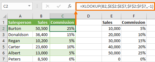
Similarly, specifying 1 in the match_mode argument will return and exact match or the next largest item.
Tip: What’s even better is that the lookup_range doesn’t need to be sorted.


The following works to return the sum of a range if your workbook/sheet doesn’t have dates available to establish the brackets of the SUM function as seen in example #5 above.
The second XLOOKUP is identical to the first EXCEPT the search mode is set to -1.
=SUM(XLOOKUP(lookup_value,lookup_array#1,return_array#1):XLOOKUP(lookup_value,lookup_array#1,return_array#1,,,-1))
Thanks for sharing, Vestal. I did a post on functions that return references just last week, which included XLOOKUP!
Thanks for your help in the past. I very much appreciate your expertise.
Currently, I am changing the date in every vlookup to get 29 different daily data points from each daily workbook for a monthly report.
One of 29 is =VLOOKUP($B$8,’J:\\REPORTS & LOGS\SHIFT REPORT\2022\12 Dec 2022\[12-1-22 Shift Report.xlsx]Copy & Paste’!$A$1:$E$31,5,FALSE). Yes, one tab is called Copy & Paste to remind others to email the summary report.
I Ctrl-C/Ctrl-V the cells of the 1st onto the 2nd and so on throughout the month. Then, I use Ctrl-H to change the dates on all 29 at same time 12-1 to 12-2 Next line 12-1 to 12-3 and so on.
Can a vlookup be automated in the monthly workbook to get data from a daily workbook by referencing a date in 1st cell on each line? A3 is 12-1-22. A4 is 12-2-22, …
If I created the whole month before all the daily reports are created, would I use IfError.
Accomplishing this task will be an AWESOME Christmas present. Thank you in advance!!!
Hi Lou,
You could use the ROW function to return a number sequence which you can append to the other components of the text string. e.g.
=VLOOKUP($B$8,INDIRECT("'J:\\REPORTS & LOGS\SHIFT REPORT\2022\12 Dec 2022\[12-"&ROW(A1)&"-22 Shift Report.xlsx]Copy & Paste'!$A$1:$E$31"),5,FALSE)If you get stuck, please post your question and sample Excel file on our forum where we can help you further: https://www.myonlinetraininghub.com/excel-forum
Mynda
How do I get a return of multiple column headers by matching a repeated row value using Xlookup? Ex. Column headers are different shopping centers and rows are different items. I am trying to look up a specific item (row) and the return to be a list of column headers (shopping centers) that sell the item. Thank you
Hard to visualise what you mean. Please post your question on our Excel forum where you can also upload a sample file and we can help you further.
Hello Mynda, I started using XLOOKUP recently and noticed many people suggesting to use lookup_array and return_array of the same size. I tried xlookup when arrays are not the same size, at times it worked well for me but sometimes it didn’t. There should be some way out of it? No one has addressed this issue. Can you also advise how to handle all types of errors in XLOOKUP.
Regards.
Hi Anand,
XLOOKUP looks up one array and finds the value on the corresponding row of the return array. If your arrays are not the same size, you will only get results when there is a corresponding row in the return array. In other words, it is a fluke that you are getting results at all. You should never use arrays of differing sizes. It simply doesn’t make sense to. I hope that helps clarify.
Mynda
Dear, Mynda
I’m trying to use the Xlookup function to sort a specific issue. But I’m stuck. Do you see a solution (or maybe another function) to use to sort this issue?
1) I have a table in the area B21:P184 (row 21 is the header row). The table lists all the games of a given baseball team during the MLB 2021 season. Each row is a separate game. The columns contains the following information from B to P; Game# (column B), Date (C), Team played against and result (D), Starting pitcher (E), and Win-Lost record for starting pitcher (F). The rest of the columns are not a part of the issue (G-P).
2) I have a separate table above (area E9:L16) (row 9 is the header row). The table lists the different starting pitchers (E), Win-Lost record (F). The rest of the columns are not part of the issue (G-L).
The issue:
I’m trying to use the xloopup function in table 2), column F, to get the latest Win-Lost record for each starting pitcher. The formula I have used is the following (Norwegian version with ; instead of ,):
=XOPPSLAG(S_RS[@[Starting pitchers]];GL_RS[Starting pitcher];GL_RS[W-L];””;1;-1)
In short; I search for the specific starting pitcher in column E in table 2 in column E in table 1, if there is a match I want the formula to give me the latest Win-Lost record for that pitcher. If the given game didn’t have a decision (the pitcher didn’t win or lose the game for his team, a reliever did) then I want the formula to search the Win-Lost record column (F in table 1) after the previous game the pitcher played and to return the Win-Lost record for that game.
The formula seems to work (if the previous game has a decision). But if the pitcher has started and pitched several games without a decision the formula won’t search any further than the previous game (this becomes a problem if the pitcher didn’t get a decision in f.ex. his last four games). If he doesn’t have a decision in a game the cell (column F in table 1) is empty. I want the formula to look as far back as to the previous decision. I hope you can help. Thank you in advance.
PS! Not sure how familiar you are with baseball, but I hope this was understandable.
Hi Anders,
It’s very difficult to hold all that information in my imagination. Would you please post your question on our Excel forum where you can also upload a sample file and we can help you further?
Thanks,
Mynda
Ok. I will do that. Thank you for the quick reply (you can delete this post if you want).
Dear Mynda
I have used Excel virtually since it was introduced (before that Lotus 123!!) and have sort of stumbled into the more advanced functions without really understanding what I was doing, like using historic sales data to produce a sales figure per postcode in the UK to see if 6 territories were fairly targeted from year to year (They weren’t). I also showed some SEO experts how to compare 6 competitors to their client using a pivot table for the organic SEO results from Spyfu. I also removed the silly assumptions that Spyfu makes and did a job that took them a month in three hours.
So, not surprisingly I love your advanced free videos and downloads and yes, I am digesting all of them.
My goal is to be able to select the course you offer such that I can complete my knowledge of Excel at the higher levels (I nearly said the highest level, but that appears to be you!!)
I have a limited budget and my goal is to become a hired hand on contract to sort out the messes which 95% of users appear to think are functional spreadsheets.
I also do LP and OR and can do the simplex equation with or without Excel Solver. I have found Optimization a difficult subject to sell to CEOs because very few of them know the first thing I am talking about, so “Nobel Prize-Winning Maths used by the Entire FTSE” just washes over them as so much soapsuds.
The spreadsheet however badly used is their friend (Or their FD’s or SD’s friend) and a simple sale plan can be turned into an optimization model without invoking black magic. If the model gets to complex, I can use FrontLine Solvers and add stats as well.
Before I can credibly do this, I need to become proficient in all of the advanced Excel features. I cannot afford all of your courses at once, so can you guide me perhaps on the best way to start after I have finished my intensive cramming on your free tutorials?
I also ought to say that I have spent 40 years in sales and marketing management and have seen every stupid reporting system under the sun. I also supplied CRM systems for 15 years (Maximizer – relational database SQL based) I am a Retired Member of the Operational Research Society, but at 66 I am anything but retired.
Thank you for your wonderful presentations – some of them have left me literally gasping or having my eyes pop out of my head.
In a couple of weeks time, I will want to start buying a couple or one course.
I would value your advice as how to proceed because my areas of interest span the lot!!
Sincerely
Steve
Hi Steve,
Thanks for reaching out and your interest in our courses.
Which course to take depends on what type of work you’re going to be doing, but if your plan is to do consulting then it’s likely your clients will be spending a fair amount of time gathering and cleaning messy data. We used to use VBA to automate these tasks, but now we can do it more quickly and easily with Power Query.
If your clients are likely to be working with big data, then Power Pivot allows Excel to work with big data spread across multiple tables like a relational database.
These ‘power’ tools are found in both Excel and Power BI, so these skills are transferable and allow you to build dynamic reports that can be easily updated.
You can get Power Query and Power Pivot in a discounted bundle with Excel Dashboards from my Excel Dashboards Course page.
Alternatively, if you want to cover general Excel skills then my Excel Expert course will cover everything from the basics (you can skip what you know) right through to the new dynamic array functions and more.
I hope that gives you some ideas. If you have further questions, please reach out via email: website at MyOnlineTrainingHub.com
Mynda
Hi,
I love your explanations, tutorials, and examples.
I really want to use the xlookup function but my excel version is 2016…..
How can I get it???
Please.
Hi Sruli, the only way to get XLOOKUP is to upgrade your Office suite to Microsoft 365.
Mam I am from India
Would you please let me know what will be the fees of xlookup course in indian currency.
The XLOOKUP tutorial here is free.
If xlookup course is free then certification is not there
There is no such certification for an individual function like XLOOKUP. Certification is only available for a more broad range of Excel skills.
hello mam, I am Anisur Rahman from Bangladesh, I am a visually impaired person I have to use only keyboard because visually impaired person can not use mouse so can I join your free course?
Hi Anisur, I imagine so. I recommend you join and give it a go. Mynda
the index and match commands are hard to understand. is there an eay way to do a vlookup with multiple criteria ? like I want a value in the table for the line where the first column is “64” AND the second column is “100”
Hi Michael,
Try this VLOOKUP multiple values technique or this VLOOKUP multiple values in multiple columns technique.
Mynda
It is an awesome explanation,
1. please tell me how you display the formula in the next cell.
2. when I got the certification please clear the process, as I am going to attempt many videos to get skilled in excel.
Thank you!
You can use the FORMULATEXT function to display the formula in a cell.
I’m not sure what you mean by the certification.
Mynda
Hello mam
I joined your free courses, as due to lockdown I have no process of payment. That’s why I was asking that the person who join the free course will be certified or not, and if certified then what will be the process.
Ah, thanks for clarifying. Sorry, our free courses don’t come with certificates as they’re only extracts of our complete course.
ok mam
thanks
So cool.
Thanks for the tutorial – really well done!
Thank you! Great to know you enjoyed it, Roger 🙂
“You can return non-contiguous columns with CHOOSE in the return_array”
Fantastic! I spent a lot of time looking for that, and was afraid I had to use the old VLOOKUP.
Glad you can make use of it 🙂
Dear Mynda
Great tutorial. However, when I download the file, using Firefox, it will not open in Excel, as it says the file is corrupt. I have tried from the email link and from the website, both fail. Is this something in my setup perhaps?
Thanks and regards
Kerry
Hi Kerry,
Sorry you’re having trouble downloading the file. It’ll be something at your end as no one else has reported this problem, and I can download it without issue. If you drop me an email (website at myonlinetraininghub.com)a I can send you the file that way.
Mynda
Thank you Mynda for the very good article and examples!
But alas, Xlookup is not yet available in our Org. 🙁
Thanks, Scott. If you’re on Office 365 it won’t be too much longer.
I clicked ‘post comment’ before congratulating you on another well-written article. A lot of work goes into these I suspect!
Thanks, Peter. Indeed, a lot of work for this one, but it’s always fun playing with a new function.
An alternative to the nested formula you attributed to Bill Jelen
= XLOOKUP( Month, MonthHeader, XLOOKUP(Item, ItemHeader, Data) )
is to look up the row and column independently and then intersect the ranges
= XLOOKUP(Item, ItemHeader, Data) XLOOKUP(Month, MonthHeader, Data)
Using direct referencing notation this is
=XLOOKUP(F2,B1:D1,B2:D13) XLOOKUP(G2,A2:A13,B2:D13)
[everyone else will find this simpler but my eyes just glaze over when I try to read the formula]
Ah yes, the space operator. Nice 🙂
I also prefer Table structured references, but I purposely avoided them for this example to make the examples easy to reference in the images.
Mynda,
Thanks, that’s really interesting.
It also solves an issue I’ve been struggling with – how to return non-contiguous columns in a dynamic array. Something like =FILTER(CHOOSE({1,2,3},A1:A51, D1:D51, F1:F51),A1:A51=10) works.
It would be better if you could just specify a list of columns in the array section of the formula, but I haven’t been able to figure out a way to do that.
Is there a better way than CHOOSE?
Thanks, Stephen. I’m not aware of a better way to return non-contiguous columns than CHOOSE. The alternative I can think of is separate FILTER formulas, one for each column you want returned.
Mynda
You can use INDEX() to reorder the columns for you and do a lookup on the result as the array in, say, VLOOKUP().
You can reorganize your lookup array as you please, including the use of non-contiguous columns (or alternatively, rows, if doing an HLOOKUP()).
For instance, data in columns A through E, you want to lookup using column D and get column A’s value:
=VLOOKUP(“mmm”,INDEX(A:E,ROW(1:5),{4,1})
The advantage to using INDEX() is largely most people are more used to using it vs. CHOOSE(), but also that CHOOSE() can produce some very odd seeming results used like this unless one is fairly particular about using it (though not in really simple situations). And it seems more “natural” somehow, when using INDEX(), which I imagine to be since it is designed for this kind of thing, whereas CHOOSE() is being used in a less intuitive manner as I think people think of it as choosing A thing, not a whole column, and choosing ONE thing, not several things, like columnS. (Reordering the coilumns (or rows) is probably equally non-intuitive for both.)
So the above demonstrates creating an ad hoc two column (the two columns of interest) table using non-contiguous columns which, since it also puts them into a different order, allows VLOOKUP() to “look left” in its search for a result.
One can even have a column more than once, but it’s hard to see much need for that. But this isn’t Soviet Russia. If you want a column to have 10 copies, then by all means (just use, say, {23, 23, 23, 4, 5, 6, 1, 19} and you have column 23 leading off as the first three columns in your output array), do it.
It doesn’t like {}’s for both rows and columns, but will take one set if you can use something else, like SEQUENCE() or the older “ROW(1:###)” technique, to generate the other selection. Using both can let you select and reorder rows AND columns giving you a subset in both dimensions for your data table. Must admit though, FILTER() would probably usually be much more straightforward for part of the work, except one must remember to select its subset outside its results, not try to create the results and use it as a feeder for further selection. That last is actually straightforward, once you think it through.
INDEX() is not my favorite function, but it does shine.
Nice! Thanks for sharing, Roy 🙂
Ahh… heaven. If they actually have reached a roll-out point. Don’t get me wrong, I’d rather wait — some — so they get it right since this is “It” for the next 30 years. But a year-and-a-half soon and… oh wait, silly me, that’s the Spill functions, sorry. But still, I’ve never read someone claiming to have it in the “wild”… not even articles like this say they have been given it. The articles only talk about logical ways to use it, not having it. Ever.
VLOOKUP did not originally have to break with column insertion or deletion as for a long time, past 2000 I believe, Excel had an option to use column and row headers as labels. Ad hoc labels, not processed as Named Ranges. Refer to the column in that way and no problema. That functionality is now simulated with the buried MATCH. History… it’s all I have yet as I wait! Hopefully they’re making the effort to get it right. It IS improved from initial announcements, including the “Not found” argument now which is both nice, and as an improvement before formal roll-out, a very good thing.
Side note: I wish they’d stop immediately giving errors when ranges do not match in size or shape. Functions should evaluate and see if the place to select a return value from is in the return value range specified. If it is, it should simply be returned rather than hammering you into the ground with a mindless failure. If the place to select the value is not in the return value’s range, THEN go right ahead and give an #ERROR. Might that make troubleshooting harder? I suppose, maybe. In a mild way. Much more valuable to get the results that ARE possible.
What that leads to I guess, is that I’d like a lot of the nanying to be removed, the “we’ll do it for you” stuff. “We’ll check… oh you silly billy, that’s not a satisfactory <> formula element. ERROR ERROR Try again puny human.” The world gets a lot of value out of imprecise things and I’d like to have functions only fail if they actually fail, OR if the failure cause will create failure INSIDE the working of the function leading it to go wildly wrong. A failure like the above would only be at the absolute end and under circumstances in which Excel knows not to return anything that, in some crazy way, did come up. So it would error only then, and only when THAT happened. Oh well… computer scientists and programmers can’t seem to understand points like that. (‘Cause it ain’t the other side of the coin: I’m not wrong here. So long as the fault affects only the end result, no interim steps, there’s no harm done.)
Come to MEeeeee XLOOKUP, come to MEeeee…
Hi Roy,
I can relate to the frustration of having to wait so long for these new features, but with over 30 million lines of code in the Excel application there’s a lot that could be impacted by such a significant change to the calc engine and they want to get it right. Given that Dynamic Arrays are now in the Insider Slow channel, it won’t be too much longer before they’re generally available 🙂
FWIW, not all functions throw errors when the ranges aren’t the same e.g. SUMIF will allow different size ranges.
Mynda