The Best Excel Functions for Dynamic References

Imagine you've built an Excel report, and everything looks great. But when you add data for the next month, your charts and formulas don’t automatically update. You’re stuck manually editing them every time you add new data.

Sound familiar? It doesn’t have to be this way! Excel offers powerful functions that return dynamic references, allowing your spreadsheets to update themselves automatically.

In this guide, we'll cover the best functions for dynamic references, making Excel do the work for you!

Watch the Dynamic References Video

 

Get the Excel Practice File

Solution 1: Using Excel Tables

One of the easiest ways to create dynamic references is by converting your dataset into an Excel Table.

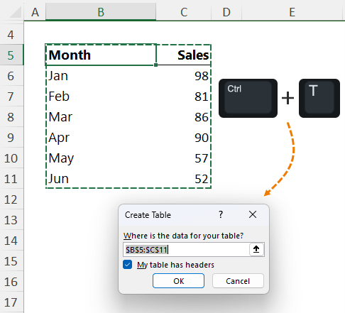
Steps to Create a Table:

1. Select your data range.
2. Press Ctrl + T to create a table.
3. If your data has column headers, ensure the "My table has headers" option is checked.
4. Click OK.

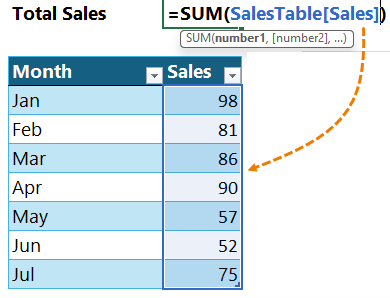
Now, when you add a new row, any formulas or charts referencing the table’s structured reference will update automatically.

However, tables don’t work well with dynamic array formulas that spill, returning #SPILL! errors:

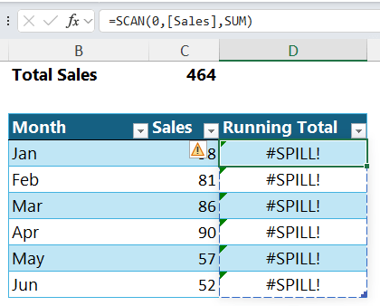
And structured references only apply to whole columns, not specific cell ranges or rows.

This is where functions that return dynamic references become essential.

Solution 2: Using Functions That Return References

Here are the best Excel functions for dynamic references which make your formulas truly dynamic.

1. OFFSET: A Classic (But Volatile) Approach

The OFFSET function allows you to return a reference that grows dynamically based on the number of rows or columns in your dataset.

Example:

I can use OFFSET inside SUM to return a dynamic cell reference for the sales by month:

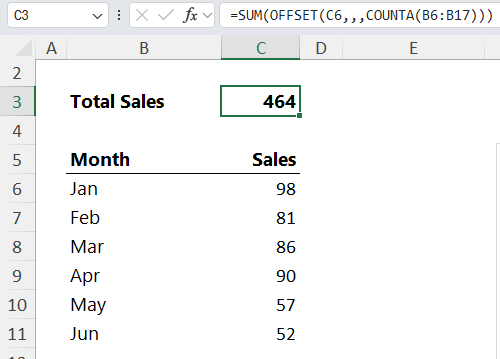
OFFSET(C6,,,COUNTA(B6:B17))

• C6: The starting cell.
• ,,: The next two arguments are skipped because no row or column shift is needed.
• COUNTA(B6:B17): Dynamically determines the number of rows based on non-empty values in column B.

Now, when you add new data, OFFSET automatically includes it. You can use this formula in SUM, charts, and other calculations.

Note: OFFSET is volatile, meaning it recalculates every time anything changes in the file, which can slow down large workbooks.

2. INDEX: A Non-Volatile Alternative

Unlike OFFSET, the INDEX function is non-volatile and recalculates only when necessary, making it a better choice for performance.

Example:

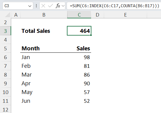
C6:INDEX(C6:C17,COUNTA(B6:B17))

• C6 is the first cell in the range to be summed.
• C6:C17: The data range to be indexed.
• COUNTA(B6:B17): Finds the number of rows in the range. This is passed to INDEX which returns the last cell containing data in the range B6:B17.

If you need a full range instead of a single value, combine two INDEX functions on either side of the colon range operator:

=SUM(INDEX(…):INDEX(…))

This approach ensures your formulas update dynamically without slowing down your spreadsheet.

3. XLOOKUP: A Lookup Function That Returns References

If you're more comfortable with lookup functions, XLOOKUP can also return a reference.

Example:

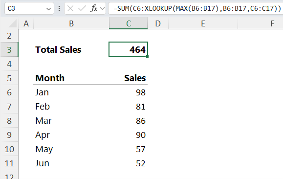
C6:XLOOKUP(MAX(B6:B17), B6:B17, C6:C17)

• C6: the first cell in the range.
• MAX(B6:B17): Finds the latest date – Note: the dates in column B are formatted to only show the month name, but the underlying cell contains the date serial number in dd/mm/yyyy or mm/dd/yyyy format.
• B6:B17: The lookup array.
• C6:C17: The return array.

XLOOKUP returns the cell reference for the sales value associated with the maximum date.

Like INDEX, XLOOKUP is non-volatile and an excellent alternative to OFFSET.

4. TOCOL: A New Function for Excel 365 Users

The TOCOL function is designed to convert multiple columns into a single column, but it can also return a dynamic reference.

Example:

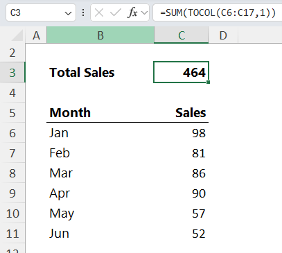
TOCOL(C6:C17,1)

• C6:C17: The range to be referenced.
• 1: Ignore blank cells.

While TOCOL doesn’t technically return a reference (it returns an array of values i.e. all values in non-blank cells in the range C6:C17), it works well inside SUM and similar functions but will not work nested in functions that require a range, like SUMIF or SUMIFS.

5. TAKE: Another Powerful Alternative for Excel 365

TAKE is another new function that simplifies returning dynamic ranges.

Example:

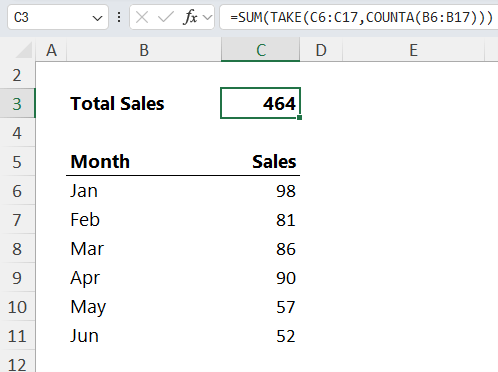
TAKE(C6:C17,COUNTA(B6:B17))

• C6:C17: The data range.
• COUNTA(B6:B17): Determines the number of rows to include.

TAKE is ideal for dynamic references without the performance drawbacks of OFFSET and unlike TOCOL, TAKE returns a reference and can therefore be used in functions like SUMIF and SUMIFS.

6. TRIMRANGE: The Future of Dynamic Ranges

TRIMRANGE is a new function that eliminates empty cells from a reference dynamically.

Example:

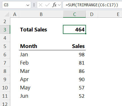
TRIMRANGE(C6:C17)

TRIMRANGE automatically removes leading and trailing empty cells, making it a better alternative to OFFSET.

For even more simplicity, use the dot operator either side of the colon instead of writing out the whole TRIMRANGE function:

=SUM(C6.:.C17)

This trims empty cells from the reference without needing a function!

Choosing the Best Function for Your Excel Version

Excel Version	Best Functions for Dynamic References
365 Beta Channel	TRIMRANGE, TrimRef Dot Operator
365 Current Channel	TOCOL, TAKE
Excel 2021	XLOOKUP, INDEX
Excel 2019 or Older	INDEX, OFFSET (if minimal use)
All Versions	Table Structured References (if spilled arrays aren’t required)

If backward compatibility isn’t an issue, go with TRIMRANGE or the dot operator in Excel 365 Beta. Otherwise, use TAKE or TOCOL for Excel 365, and INDEX or XLOOKUP for older versions.

Conclusion

By using these functions, you can:

• Avoid broken formulas.
• Eliminate manual updates.
• Make your spreadsheets more efficient and reliable.

Mastering dynamic references means spending less time fixing formulas and more time getting valuable insights from your data.

Next Steps

To learn more about these powerful functions and other advanced Excel techniques, check out our Advanced Excel Formulas Course for step-by-step guidance and expert mentoring.

Enroll Now and take your Excel skills to the next level!

If you found this guide helpful, make sure to share it with others who might benefit from dynamic Excel formulas!