Extracting subsets of data from large datasets is crucial for making informed decisions. However, manually filtering data can be time-consuming, especially when working with dynamic datasets that frequently update.
In this guide, we’ll explore a powerful Excel combo that automates real-time data extraction from one sheet to another as shown below, making it easier to track sales, manage inventory, and analyze employee records to name a few:
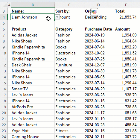
Table of Contents
- Watch the Video
- Get the Free Excel File
- Step 1: Formatting the Data
- Step 2: Creating a Unique List
- Step 3: Setting Up the Drop-down List
- Step 4: Filtering Data Dynamically
- Step 5: Sorting the Extracted Data
- Step 6: Adding Sort Order Option
- Step 7: Calculating a Dynamic Total
- Alternative Method for Earlier Excel Versions
- Next Steps
Watch the Video

Get the Free Excel File
This workbook has the completed example that extracts data from one sheet to another so you can modify it for your own needs:
Enter your email address below to download the sample workbook.

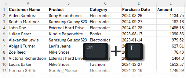
Step 1: Formatting Data as a Table
Before we start, it’s best to format our dataset as an Excel Table. This ensures that any new data is automatically included in our filters.
Shortcut: Press CTRL + T to convert data into a table.
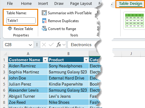
Once formatted, Excel assigns a default table name, which can be modified in the Table Design tab:
Step 2: Creating a Unique List for Data Validation
To dynamically filter data, we need a unique list of customer names for a drop-down list.
Use the UNIQUE function wrapped in the SORT function to extract and sort unique customer names:
=SORT(UNIQUE(Table1[Customer Name]))
Note: Table1[Customer Name] is a Table Structured Reference. These make it easier to see which data is being referenced, and they automatically adjust when new data is added.
Step 3: Setting Up the Drop-down List
To create a drop-down list for easy selection, follow these steps:
- Insert a new sheet for the filtered data.
- Select an empty cell (I used cell B4), go to the Data tab → Data Validation → List.
- Use the unique customer list on the Data tab as the source: =Data!$G$2#
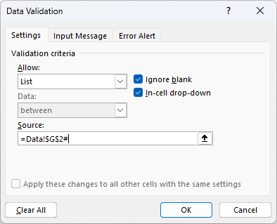
The # (hash sign operator) dynamically references the entire spilled array returned by the UNIQUE formula created in step 2, ensuring that any new customers added to the table are automatically included in the data validation drop-down list.
Step 4: Filtering Data Dynamically
Now, we use the FILTER function to extract relevant data based on the selected customer:
=FILTER(Table1[[Product]:[Amount]], Table1[Customer Name]=B4, "No purchases found")
- Array: The range we want to extract.
- Include: Filters rows where Customer Name matches the selected value.
- If_empty: Displays a message if no data is found.
When a new customer is selected, the data updates automatically.
Step 5: Sorting the Extracted Data
To sort the filtered data, follow these steps:
- Add a drop-down list in C4 to choose sorting criteria (e.g., the columns returned by filter including Amount, Date etc.).
- Wrap the FILTER formula in the SORT function:
=SORT(FILTER(Table1[[Product]:[Amount]], Table1[Customer Name]=B4, "No purchases found"), XMATCH(C4,B6:E6), -1)
- XMATCH(C4, B6:E6): Finds the selected column index.
- -1: Sorts in descending order.
Step 6: Adding Sort Order Option
To toggle between ascending and descending order:
- In D4, create a drop-down list with Ascending and Descending.
- Modify the SORT function:
=SORT(FILTER(Table1[[Product]:[Amount]], Table1[Customer Name]=B4, "No purchases found"), XMATCH(C4,B6:E6), SWITCH(D4,"Ascending",1,"Descending",-1))
The SWITCH function converts text selections into numeric sort orders.
Step 7: Calculating a Dynamic Total
To calculate the total Amount dynamically:
=SUM(CHOOSECOLS(B7#,4))
- B7#: References the spilled array.
- The CHOOSECOLS function extracts the 4th column (Amount) from the array.
This method ensures that the total updates to include all results when the customer name selected changes.
By combining SORT, FILTER, UNIQUE, and SWITCH functions, we’ve built a dynamic data extraction tool that updates in real-time. This method saves time and enhances decision-making efficiency.
Alternative Method for Earlier Excel Versions
For users with Excel 2019 or earlier, PivotTables offer a similar solution for extracting data from one sheet to another:
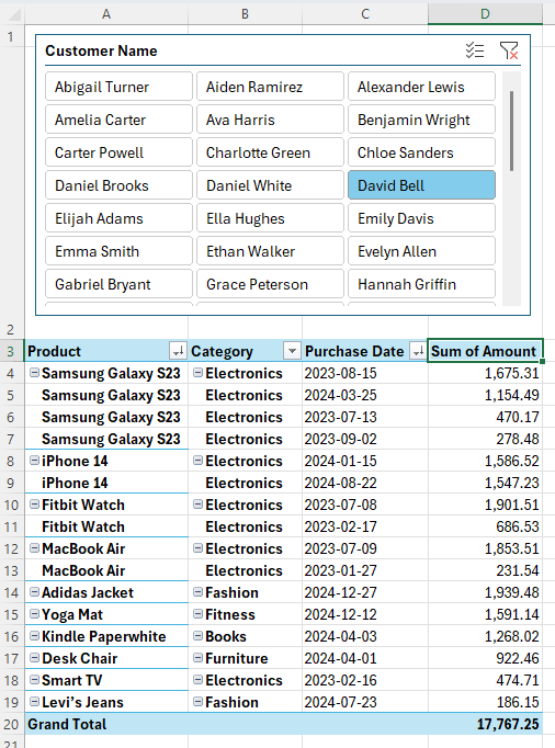
- Insert a PivotTable on a new sheet.
- Add:
- Row Labels: Product, Category, Purchase Date
- Values: Amount
- Change the report layout to Tabular, remove subtotals and enable repeated item labels via the Design tab.
- Insert a Slicer for Customer Name to filter data easily.
- Right-click on Sum of Amount and sort largest to smallest.
This provides a flexible, interactive summary without complex formulas.
Next Steps
Want to learn more? Check out our Advanced Excel Formulas course for step-by-step guidance on mastering Excel’s most powerful functions!
