Typically if you need to lookup a value from a table you'd employ VLOOKUP or INDEX/MATCH.
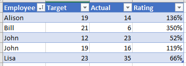
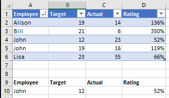
However if your data looks like this
and you are looking up by Employee name then you'll run into some issues because there are two employees with the name John.
Both the VLOOKUP and INDEX/MATCH approach will have problems with this because they need to lookup unique values.
You can use VLOOKUP or INDEX/MATCH to lookup multiple values across multiple columns but this requires writing a complicated (legacy) array formula using CTRL+SHIFT+ENTER
So, what to do? If you have the new FILTER function you could use that.
FILTER allows you to return all records that match your criteria, so in this case you could return the data related to both John's. But if you are just interested in the John with the highest Rating, FILTER will also allow you to specify additional criteria to give you the data you are after.
The key here is that FILTER lets you look for more than one thing in your source data (for example Employee="John" and Target=12) and return the data in that record.
Most people don't yet have FILTER though so this is where DGET comes in.
DGET allows you to look up a value in a table (or a range/list of records) based on multiple criteria, just like FILTER. However DGET only returns a single value, not an entire row of data.
Excel Dynamic Arrays
FILTER is one of the new Excel Dynamic Arrays family of functions.
Dynamic Arrays are currently only available in Office 365 to a portion of Office Insiders.
Excel 2019 will not have the Dynamic Array functions.
DGET Syntax
The syntax to use DGET is
where the arguments are
- database - a table/range including headers.
- field - field/header name or numeric column index.
- criteria - criteria range including headers.
DGET Examples
As shown previously I have a table of data like this, I've named the table Employees. Note that your data does not have to be in a table for DGET to work.
We have two employees named John. As stated earlier, neither VLOOKUP nor INDEX/MATCH can be relied upon to return the correct result if we want to look up something related to one of the John's.
Putting Stuff Under Tables
If you put data or formulae under a table and rows are added to the table, your data/formulae will get shifted down. This may or may not break something on you so be aware.
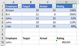
If I try to use DGET to lookup the Rating for John, it returns a #NUM! error because it doesn't know which John I want.
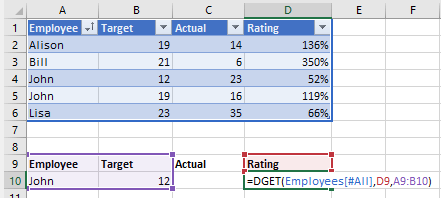
So I also specify Target is 12 and I get the answer 52% for the Rating.
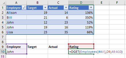
Notice that when specifying the criteria you must include the header/name of the column as well as the data, this is why the 3rd argument is the range A9:B10.
The 2nd argument for DGET is the data/field you want the function to return. In the example above I reference cell D9 which contains the word Rating, so I want the Rating returned.
I could replace the word Rating with the number 4 to indicate I want the data in the 4th column of the table returned. Of course you could just type in 4 to the DGET formula rather than reference cell D9.
Criteria
Expressions can be used in criteria such as
| Jo* | Matches a string starting with "jo" (case insensitive) |
| 12 | Equal to 12 |
| <>12 | Not equal to 12 |
| <12 | Numbers less than 12 |
| <> | Not blank |
| < 28/10/2008 | Dates before October 28 2008 |
String matching is case insensitive so "John" will match "John" and "JOHN".
Multi-Row Criteria
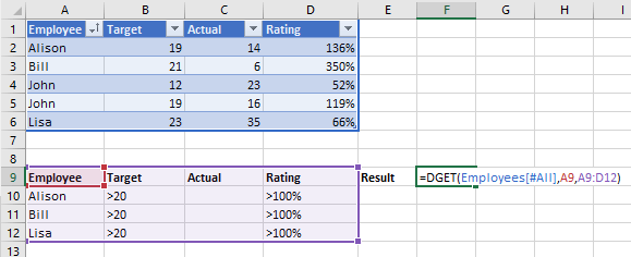
The criteria for DGET can include more than one row below the headers.
In such a scenario, the conditions in a row are joined using AND, and each row is joined using OR.
Taking the example image above, I am looking for the employee (either Alison, Bill or Lisa) whose Target is greater than 20 and whose Rating is greater than 100%.
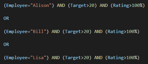
So the criteria we have are
If we check these against the source data table, we find that there is an Employee named Alison (TRUE), her Target is not greater than 20 (FALSE) and her Rating is greater than 100% (TRUE).
Doing this for all 3 rows we can simplify to
Combining the conditions within each row to give a True/False we get
The only criteria that gives a True result is the 2nd one so the value returned by DGET is the Employee that matches that, Bill.
Download Sample Workbook
Enter your email address below to download the workbook.
Examples of using DGET from this post are in the sample workbook.




How to drag dget function in row such as vlookup?
I
Not sure what you mean?
Thanks for explaining this function! I’m currently using a VLOOKUP that uses “Employee Name” to return their “Position Number”. My challenge is that sometimes my source document name is different than my position number workbook. For example, my source document lists the name as Brown, Mary and my position number spreadsheet has the name as Brown, Mary J, which returns a “N/A error because of the middle initial. Can you suggest the best VLOOKUP-type formula that will work in this scenario without using Text to Columns and the CONCATENATE formula? Thanks for your help.
Hi Annie,
The best solution is to get your source data to match your other workbook, rather than modifying formulae to accommodate multiple variations of a name. Can’t the source be restricted to ensure data is consistent? Really that is the best approach.
Regards
Phil
Thank you, Phil, this is very helpful and I’m anxious to test this a bit more. We have Office 365, but I’m not sure why the FILTER function is not available. Anyway, for DGET, my first question is does the criteria have to be in a table/range or can it be manually entered? And if so, do you have some information on the syntax for entering the criteria directly into the formula?
Hi Rob,
You have to supply a range as the criteria, you can’t manually type it into the formula.
FILTER is currently only available to some Office 365 subscribers. See the blue info box ‘Excel Dynamic Arrays’ at the top of the post for more information.
Regards
Phil
ok great, thanks!
I tried duplicating the DGET example from your sheet and it didn’t work (#VALUE!).
I was wondering why you put the “[#All]” after the table name, so I ignored it and just used the name of the table by itself. It seems that the [#All] section part of the table identifier is absolutely necessary!
Adding it with Intellisense is easy and it also exposed me to the other values (#All, #Data, #Headers, #Totals), so thanks for that tidbit.
The mulit-row criteria example is very similar (identical?) to the Advanced Filter capability with AND and OR functionality.
Great tip!
Hi Patrick,
[#All] is required because DGET needs the entire table, including headers, not just the data. Using just Employees would be referencing just the data in the table.
See Table Structured References for more info.
Regards
Phil
Thanks so much for sharing, Philip! Before reading this article, I was using SUMPRODUCT in a similar fashion to find what I was looking for when I had multiple criteria. However, it didn’t work if there was a single non-numeric value in the column that I was trying to pull results from (so in your example, if there was a NULL or #DIV/0 error in column D).
I really appreciate that this will work for non-numeric values as well. My question is this, if I want to find multiple results (for example, for both John and Lisa each), I would have listed them in separate rows and then used the SUMPRODUCT formula with appropriate references to grab their respective results; what would be the best way to write the formula for the second person since I need to include the header?
(So pretend with me that we are using the first example. I would keep row 10 to find one of the John’s information. Then, I would have Lisa’s name in A11, with 23 in B11; what would be the formula in D11?)
Thanks in advance!
No worries Choua, glad you find this useful.
Your question hits upon one of the limitations of DGET, and why FILTER is better in such a scenario. Because you have to provide the Header/column name in the criteria, doing this over multiple lines is difficult.
Before I answer your qs, I should say it’s best not to put anything below the last row of a table. In fact it’s best not to put anything below a table in case more rows are added, I’ve only done this in these examples to make demonstration easier.
But, with your example, let’s say you have your criteria like this starting in Row 12
You can’t add Lisa to Row 14 because the Header row is row 12. You could either use a data validation list in A13, B13 etc showing the data from the Employees table. Changing these will change the result you get in D13.
Or you will have to add another row of Headers like so
Regards
Phil