Reducing Data Validation List

Creating a reducing Data Validation list is easy with the new dynamic array formulas.

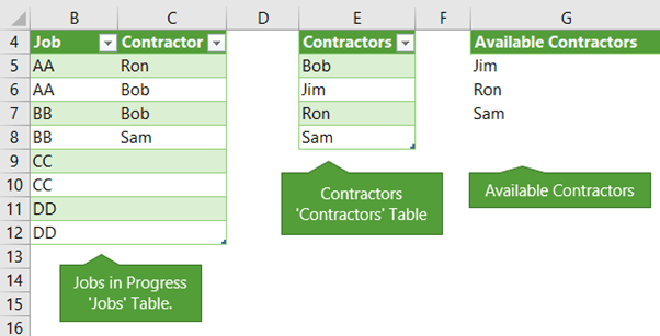
Let’s say we have a list of jobs currently in progress (column B in the image below). Each contractor can work on no more than two jobs and we have four contractors available (column E).

As we assign contractors to jobs in column C, the data validation list should reduce to only show available contractors (column G).

Note: This technique requires Dynamic Array formulas which are currently only available to Office 365 users on the Insider Channels.

Download Workbook

Watch the Video

Creating a Reducing Data Validation List

We can create reducing data validation lists in three easy steps:

Step 1: Prepare your data – I’ve given my tables names; Jobs and Contractors. Note: the dynamic array formula in column G cannot be stored in a table.

Step 2: Extract a list of available contractors - In cell G5 we use the FILTER function to extract a list of Contractors that are still available i.e. contractors that aren’t already assigned to two jobs in column C.

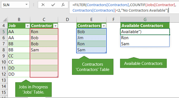
The formula, which uses Excel Table Structured References to reference the cells in the tables is:

=FILTER(Contractors[Contractors],COUNTIF(Jobs[Contractor], Contractors[Contractors])<2, "No Contractors Available")

In English it reads:

Return a filtered list based on the list in the Contractors column of the Contractors table (column E), if the count of Contractors in the Jobs table (column C) that matches the Contractors column in the Contractors table (column E) is less than 2. If there are no contractors left that meet the criteria, return the text ‘No Contractors Available’.

Notice that the formula spills the results to the cells below.

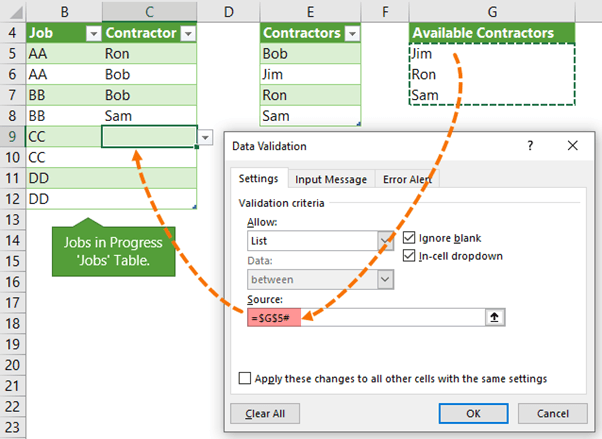
Step 3: Insert data validation list in cells C5:C12 that references the list returned in step 2. The trick when referencing a spilled range returned by a dynamic array formula is to use the spilled range operator, #, as shown in the data validation ‘Source’ field below:

That’s it, you’re all set.

Modify for Single Use

If you only want the contractor assigned to one job, simply modify the formula like so:

=FILTER(Contractors[Contractors],COUNTIF(Jobs[Contractor],Contractors[Contractors])<1,"No Contractors Available")

Likewise, if you want to assign them to 3 or more jobs, simply change the value in the logical test.

Error Checking

You’ll see that the second instance of the names returns a formula error warning, as shown in cell C7 below:

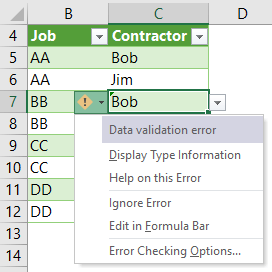
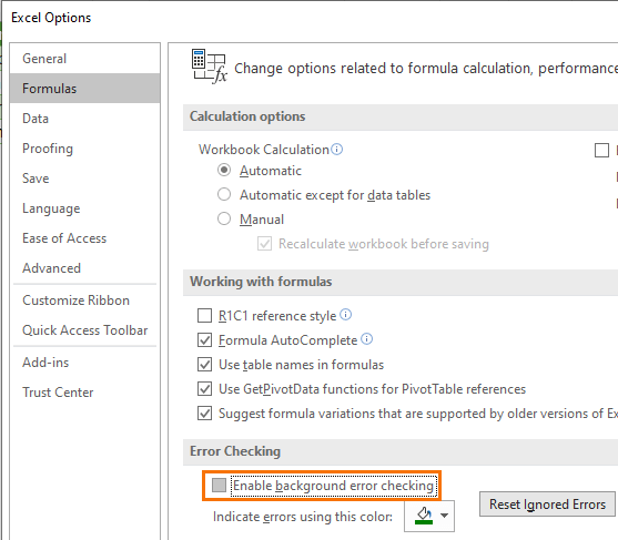
This is being returned because once you use a name twice it is no longer in the data validation list in column G. You can simply ignore the errors, or you can turn off the green indicators via the File tab > Options > Formulas:

Thanks

A special thanks to MF Wong for his original solution and to Tony Barker for asking how to extend the example to multiple uses.