Excel Shortcut When Using Dates as Formula Criteria

Working with Dates in Excel can be frustrating because a date criteria in one formula doesn’t always work in another.

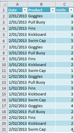
Using the data below let’s say we want to summarise units sold by Product for January.

Note: the data above is formatted as a Table which means we can use Structured References in our formulas instead of cell ranges. Click here to read how Structured References work.

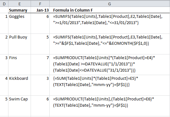
Below are 5 different formulas that all summarise the data in our table based on the criteria in column B and the date in Column A.

Notice the different ways the Date criteria is entered in each formula?

Let’s look at the pros and cons for each one.

1. SUMIFS Formula with Fixed Dates

=SUMIFS(Table1[Units],Table1[Product],E2,Table1[Date], ">=1/01/2013",Table1[Date],"<=31/01/2013")

Pros:

• SUMIFS is an easy formula to use.

Cons:

• Dates are hard keyed which means the formula isn’t dynamic. Formula # 2 is better.
• If you only have Excel 2003 then you don’t have the SUMIFS Function. Use options 3, 4 or 5 instead.

2. SUMIFS Formula with Dynamic Date Reference

=SUMIFS(Table1[Units],Table1[Product],E3,Table1[Date],">="&$F$1,Table1[Date],"<="&EOMONTH($F$1,0))

Pros:

• Same as formula # 1 plus the date criteria is linked to a cell which means if the cell changes you don’t need to change the formula, and if you want to summarise February, March.... you can simply insert columns beside F and copy the formula across without having to update it.

Cons:

• SUMIFS isn’t available in Excel 2003.

3. SUMPRODUCT Formula with Fixed Dates

=SUMPRODUCT(Table1[Units]*(Table1[Product]=E4)*(Table1[Date] >=DATEVALUE("1/1/2013"))* (Table1[Date]<=DATEVALUE("31/1/2013")))

Pros:

• SUMPRODUCT works in Excel 2003 onwards

Cons:

• Hard keyed date means it’s not dynamic.
• Need to use the DATEVALUE function for Excel to interpret the date criteria correctly.

4. SUM array formula

{=SUM(Table1[Units]*(Table1[Product]=E5)*(TEXT(Table1[Date],"mmm-yy")=$F$1))}

Pros:

• This array formula works in Excel 2003 onwards
• Dynamic date reference to cell F1
• Only one date criteria is required. Using TEXT(Table1[Date],"mmm-yy") tells Excel to find all dates for the month of Jan-13 so we don’t need to specify ">=1/01/2013" and "<=31/01/2013".

Cons:

• It’s an array formula which means it’s not the most efficient formula, plus some people don’t understand how array formulas work so it is susceptible to human error.
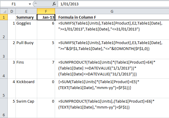
• We need to enter the date in cell F1 as text. See how the date in the formula bar below is preceded by an apostrophe, yet in the cell you can’t see it. This apostrophe forces Excel to interpret the value as text.

What is interesting is this format works in all of the above formulas, but if you were to enter the date like this: 1/01/2013 and format it as mmm-yy using cell formats, then formulas 4 and 5 don’t work – see below:

5. SUMPRODUCT Formula

=SUMPRODUCT(Table1[Units],(Table1[Product]=E6)*(TEXT(Table1[Date],"mmm-yy")=$F$1))

Pros:

• Works in Excel 2003 onwards.
• Dynamic date reference to cell F1.
• Only one date criteria is required like the SUM array formula above.
• It’s not an array formula.

Cons:

• Requires the date in cell F1 to be entered as text.

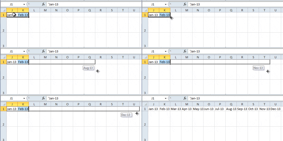
The downside with formatting the date criteria as text is you can’t use AutoFill because Excel doesn’t recognise the series.

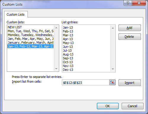
However if it’s something you’re going to use regularly you can set up a custom AutoFill list.

Excel 2007 > Windows button > Excel Options > Popular > ‘Edit Custom Lists’ > Add a new list

Excel 2010 > File tab > Options > Advanced > General > ‘Edit Custom Lists’ > Add a new list.

Now when you type in the first two months from your series you can use the AutoFill button to drag and fill the remaining dates.

A special thanks to Martin Cronin for sharing his TEXT(Table1[Date],"mmm-yy")=$F$1) trick with me.

If you liked Martin's tip please show your appreciation by sharing it using the social media links below.