This Excel Factor tip was sent in by Roberto Mensa of Italy.
Words by Mynda Treacy.
Data validation lists are a great way to control the inputs to your worksheets and having one list dependent on another is nothing new. I did a post on how to do this using a named range trick.
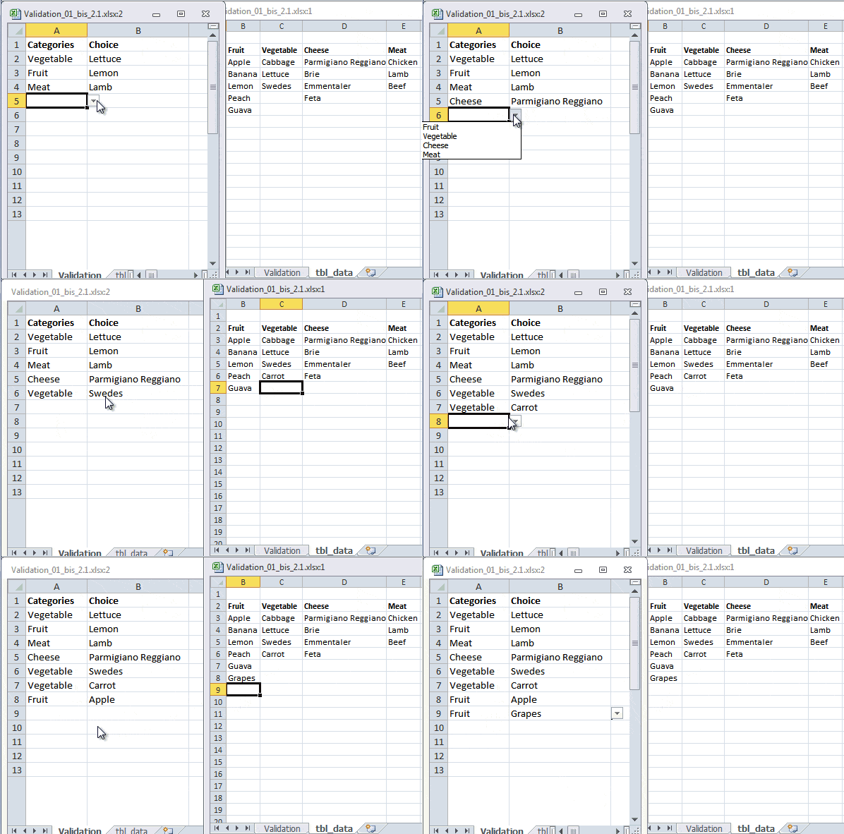
But, Roberto’s solution is better because it’s dynamic, and that means you can change the names of the lists, or add new items to the lists and it will automatically include them in the data validation list like this:
Let’s take a look at how Roberto uses some clever Named Formulas with data validation to dynamically generate the lists.
How to set up Dynamic Dependent Data Validation Lists
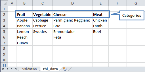
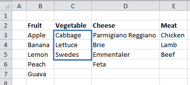
The lists are on a sheet called tbl_data in cells B2:E7. Row 2 contains the categories. This is the primary list (it will be called ‘Categories’) and rows 3:7 contain the secondary lists (they will be called ‘Choice’).
Step 1
First define a Named Formula for the Categories. To do this go to the Formulas tab of the ribbon and select ‘Define Name’.
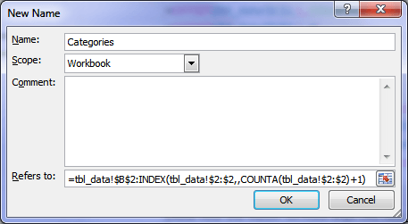
Name it ‘Categories’ with the scope ‘Workbook’ and in the ‘Refers to:’ field enter this formula:
=tbl_data!$B$2:INDEX(tbl_data!$2:$2,,COUNTA(tbl_data!$2:$2)+1)
Like this:
This creates a reference to the column headers for the primary list. i.e. Fruit, Vegetable, Cheese, Meat.
The INDEX and COUNTA functions in the formula count how many cells contain data in row 2, whereby generating a dynamic range for the named formula. The +1 on the end is to account for the blank cell A1.
This means if you add another list of data in column F it will also be automatically included in the data validation lists.
Step 2
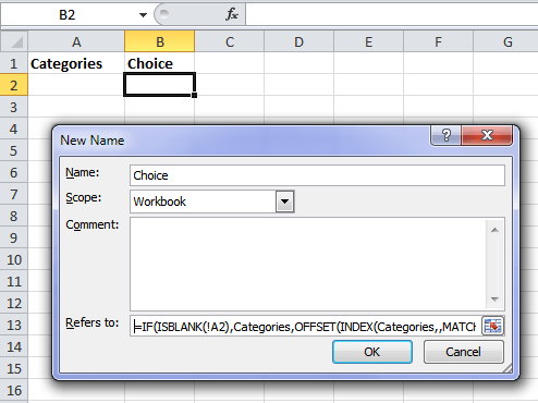
Step 2 is much like step 1 in that you set up another named formula. This time it is called ‘Choice’.
This named formula is used to generate the validation list for both the ‘Categories’ in column A and the ‘Choice’ in column B.
This formula behaves differently depending on which cell you have selected and the value in the cell immediately to the left.
To understand how it works we’ll look at it from the point of view of cell B2, where it is identifying the category in cell A2….:
And then finding the corresponding list on the tbl_data sheet for ‘Vegetable’:
Here’s the formula:
=IF(ISBLANK(!A2),Categories,OFFSET(INDEX(Categories,,MATCH(!A2,Categories,)),1,, COUNTA(OFFSET(INDEX(Categories,,MATCH(!A2,Categories,)),1,,100))))
See how the cell references have an exclamation mark before them - !A2. This exclamation mark acts like a relative reference and allows you to use the same validation anywhere in the workbook.
Note: this referencing style is only allowed in the name manager.
This referencing style also means you need to select cell B2 before you set up the named formula like this:
And now to understand what the formula is doing (in English):
Warning: You might like to get some coffee or Red Bull before reading this part!
Essentially, Roberto has used the OFFSET function to generate a range for the list of vegetables.
Here is the formula again so that it’s easy easier to cross reference the syntax to the English translation:
=IF(ISBLANK(!A2),Categories,OFFSET(INDEX(Categories,,MATCH(!A2,Categories,)),1,, COUNTA(OFFSET(INDEX(Categories,,MATCH(!A2,Categories,)),1,,100))))
And in English:
IF cell A2 is blank, then list the Categories, otherwise, find the range of cells that contain the list for the matching category. Start by finding the first cell in the range, which will be the cell that matches the value in A2 in the Categories list (tbl_data!C3), then go down one row but stay in the same column, then count the number of cells that contain data, again by finding the cell in the Categories list that matches the value in A2, then go down 1 row and count the number of cells containing data for the next 100 cells, this will give you the last cell in the range (tbl_data!C5).
Below are the functions used in the above Named Formula and their syntax. Click on the links if you want the English translations for the functions below:
OFFSET Function
=OFFSET(reference,rows,cols,[height],[width])
Note: I’ve crossed out the ‘cols’ and ‘width’ arguments in the OFFSET function because these are omitted in Roberto’s formula as they’re not required.
INDEX Function
=INDEX(reference,row_num,[column_num],[area_num])
There are two forms of the INDEX function: the array form which has the syntax INDEX(array,row_num,column_num), and the reference form (syntax above). In this formula Roberto has used the reference form.
The INDEX function in reference form returns the reference of the cell at the intersection of a particular row and column.
Note: I’ve crossed out the row_num argument because when an array contains only one row the corresponding row_num argument is not required. Remember the ‘Categories’ are only in row 2 on the tbl_data sheet.
The area_num argument is also crossed out because it is not required since the formula only references one area, which is ‘Categories’.
MATCH Function
=MATCH(lookup_value,lookup_array,[match_type])
COUNTA Function
=COUNTA(value1,[value2]….)
Let’s step through the evaluation of the formula in cell B2:
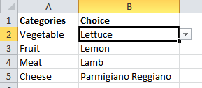
Remember, in cell A2 we have selected ‘Vegetable’ like this:
Step 1 evaluate the 1st INDEX & MATCH formula; what is the value in A2 and what range is it looking in:
=IF(FALSE, Categories, OFFSET( INDEX(Categories,,MATCH("Vegetable",tbl_data!$B$2:$E$2,)),1,, COUNTA( OFFSET( INDEX(Categories,, MATCH("Vegetable",Categories,)),1,,100))))
Step 2 finish evaluating the 1st INDEX & MATCH formula and start evaluating 2nd INDEX & MATCH formula; convert remaining Named Formulas to cell references:
=OFFSET(tbl_data!$C$2,1,, COUNTA( OFFSET( INDEX(tbl_data!$B$2:$E$2,, MATCH(A2,tbl_data!$B$2:$E$2,)),1,,100)))
Step 3 evaluate the 2nd MATCH formula; what is the array and what column_num is the list in:
=OFFSET(tbl_data!$C$2,1,,COUNTA(OFFSET(INDEX(tbl_data!$B$2:$E$2,,2),1,,100)))
Step 4 complete evaluating the INDEX formula:
=OFFSET(tbl_data!$C$2,1,,COUNTA(OFFSET(INDEX(tbl_data!$C$3:$C$102),1,,100)))
Step 5 evaluate the OFFSET formula:
=OFFSET(tbl_data!$C$2,1,,3)
Step 6 voila. The range containing the list for Vegetables:
=tbl_data!$C$3:$C$5
Setting up the Data Validation Lists
This is the easy part!
- Highlight the cells in both column A and B that you want validated.
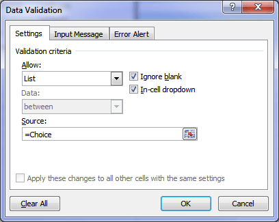
- Data tab of the ribbon > Data Validation > Allow: List > in the ‘Source:’ field enter =Choice
Summary
Phew…there is a lot to take in with that tip but there are a few key points that I think are worth recapping:
- You can use the exclamation mark in the name manager to create a relative reference to a cell e.g. !A2. But only in the name manager.
- INDEX function; If a reference contains only one row or column, the corresponding row_num or column_num argument is optional.
- There is only one named formula that validates both the ‘Categories’ and the ‘Choice’ – clever eh!
- You can use this named formula in any worksheet in your workbook.
- Using this approach allows the greatest flexibility in your lists. Both categories and choices can be added or changed and they will dynamically feed through to your data validation lists.
Enter your email address below to download the sample workbook.
One Last Thing...
As an alternative you can set your lists up in a Table and take advantage of the structured references with a formula like this:
=IF(ISBLANK(!A3), MyTbl[#Headers], OFFSET(INDIRECT("MyTbl["!A3&"]"),,, COUNTA(INDIRECT("MyTbl["!A3&"]"))))
Download the second workbook and take a look at how it works.
Update
In response to a question in the comments below from Mike, Roberto has taken this trick to the extreme and created a way to allow new items to be added to the data validation lists on the fly.
Take a look at his magical solution here on his blog.
Incredibly it doesn't even require VBA.
Thanks for sharing this tip, Roberto.
You can see more of Roberto’s Excel work at E90E50 and E90E50fx. And for the last year he has published articles with the Frankens Team.
Vote for Roberto
If you’d like to vote for Roberto's tip (in X-factor voting style) use the buttons below to Like this on Facebook, Tweet about it on Twitter, +1 it on Google, Share it on LinkedIn, or leave a comment to thank Roberto for taking the time to suggest this tip….or all of the above 🙂



This is great, thanks. One problem I’m coming across though is when a user changes the category they’ve selected after they have selected their choice. For example, they select ‘Fruit’ in column A and then ‘Apple’ in column B but then go back and change ‘Fruit’ to ‘Vegetable’. ‘Apple’ still remains in column B so they think they’ve made a valid selection. Is there a way to remove the option in column B if the selected option in column A changes?
Hi Roxanne,
You can’t have it auto delete the invalid selection, but you can use conditional formatting to highlight it in red and draw attention to it, so the user knows to fix it.
Mynda
Hi, many thanks for publishing this dynamic data validation list. Is there a way to add a third validation list that is linked to both the categorie and choice lists?
Hi Rob,
Yes, you can see this example of a dependent data validation list.
Mynda
HI Mynda, thanks ever so much in taking the time to reply, I have limited experience in excel and I am only at the beginning of the learning journey. My problem is that the sheet I need is to pick a drop down list of any of 5 wind farms, that then gives any of a dozen wind turbines at that farm, that then gives an I.P address to a particular turbine that can then has the option to goto that turbine i.p address by opening a browser. when I try to transpose that data the sheet drop down lists stop working.
Its back to the drawing board as I obviously need a lot more excel learning
You’re welcome, Rob. If you’d like us to take a look you can post a sample Excel workbook and your question on our Excel forum and we can help you troubleshoot.
Mynda
Thanks for this great technique. I have a small question. Some people manage to make the word choose.. appear on the data validation box when no selection has been done in the drop down. The word choose.. appear even when you attempt to delete it. Can you please help me figure out how to do that? Thanks
Hi Ufoo,
Press Alt+F11 to open the visual basic editor, and look into that sheet vb module. That can be done with a code.
Dear Sir,
Could Roberto or another Excel Genius, please show me how to add items to Sheet 2 (tbl_data), by just inputting the new item in the Choice column of Sheet 1 (Validation), after selecting the respective Category? eg: If we select Vegetable under the Category column, the Choice column drop-down only shows Cabbage, Lettuce & Rutabaga, but I want to add Tomato, and want to do it “on-the-fly” by inputting the word “tomato” in the Choice cell. Then the program will ask if I want to add the new item to the list. I select “Yes”, then it adds it to the list of vegetables on Sheet2, and sorts in alphabetical order. I do not want to have to switch from Sheet 1 to Sheet 2 to add a new item. Debra Dalgleish of Contextures has got examples of drop down lists updated “on-the-fly”, but not for dynamic dependant drop-down lists. I appreciate your help.
Hi Mike,
Roberto has provided a truly magical solution in this .xlsx file.
I haven’t had time to decipher it and see how he has worked his genius, but I’m sure if you spend some time following the formula trail you will figure it out.
Kind regards,
Mynda.
thanks a lot….that was Great!
On behalf of Roberto, you’re welcome 🙂
if i modified value in list item, its been reflecting to my list.. but its not modifying on selected value of dropdown list.. what to do for this?
Hi Phani,
Excel remembers the selected value in a data validation list despite the list changing. It will not update until you select the data validation list and make a new choice.
Kind regards,
Mynda.
Hi
I am using the below table 1 named as product and used as reference for data validation in table 2. having 2 sub categories in (Table 2): Fruit and Vegetables.
Table 1
FRUIT VEGETABLES(Named :-Product)
Apple Carrot
Banana radish
Lichi Peas
Papaya Cabbage
Table 2:
product Type
Fruits Apple
Vegetables Carrot
In table 2, I am getting exact type of product as per the option selected in product column for fruit and vegetables.
I want a cost of a product and it’s type selected in third column under heading cost, in Table 2. I update my table 1 to table 3 including cost of every item.
Table 3
Apple 100 Carrot 10
Banana 50 radish 20
Lichi 65 Peas 30
Papaya 80 Cabbage 40
By using if function I am getting value for all the selected items of fruit only in cost column but not for vegetables and vice versa, I am trying (Or with if function), Kindly help me which function I can use so that I can get the
product—–> Types—-> Cost, as per the selection made in the product and type column to get the respective cost.
Thanks & Regards.
Ajay
Hi Ajay,
If you’ve got your dependent data validation working and all you need to do is lookup the cost of the fruit or vegetable then I’d just use a VLOOKUP or INDEX & MATCH formula to find the cost.
If I’ve missed something please let me know.
Kind regards,
Mynda.
hi
I have gone through some tutorials, where they make use of Substitute and offset function along with dependent list, but I do not reach to the level to make that understand. Kindly help.
Thanks & Regards.
Ajay
Hi Ajay,
Perhaps if you could give me an example of this formula I can help you understand what it’s doing?
Kind regards,
Mynda.
hi ,
thanks for sharing these useful tips about excel`s validation list , i have a problem here actually that am not able to find a way to link between 3 columns with validation lists , where the 2nd and 3rd column is dependent on the value shown in the first validation column ,
for example :
column 1 column 2 column 3
“item description” “size” “end connection”
pipe 1-10( for pipe) (range from xx to yy )
elbow 30-40(for elbow) ( range from aa to bb )
reducer 60-70 ( for reducer ) (range from cc to dd )
what i want is the following :
when column 1 validation list shows (pipe) , column 2 shows size from ( 1-10 ) & column 3 shows range from xx to yy
i used the INDIRECT function to link between columns 1 and 2 but i failed to find anyway to link the 3 columns as i mentioned above .
Any help guys ???
Hi Mr. Joe,
Please send your file and description to us and we can have a look at it for you : Help Desk
Cheers,
CarloE
WOW – Been breaking my head trying to learn lookup functions, validations, lists, etc., so much more to excel than I’ve used, and it’s all so useful! I got stuck and frustrated when INDIRECT no longer worked when I learnt about dynamic named ranges. This is exactly what I’ve needed to ‘bring it all together’, took awhile to find this blog, but happy I did. Thanks again for being brilliant and sharing that with us!
Hi Steve,
You’re welcome on behalf of Mynda.
Cheers,
CarloE
Just what I needed!!!
Will save me hours of time
Hi Greg,
Cheers!!!
CarloE
Its very usefull for who those are use MS-Excel.
Cheers, Rao 🙂
Super! Any idea if and how I can implement this on google spreadsheets?
Hi Harshad,
That’s a very interesting question. However, I went to google and tried to simulate it there
and it’s disappointing that Named Ranges in Google Spreadsheets can’t accept Formulas as reference.
So I guess, that’s it.
Cheers.
CarloE
Hi, this is really an amazing tip. However, (just to be complicated) my range of items that is picked up in the drop contains null values i.e formulas returning a zero. These are being picked up in the drop down. Is there any way to exclude these?
Hi Edgar,
Yes there is. It would be easier to give you a solution if you can send me your file. You can attached it if you raise a ticket in our help desk.
Thanks,
Mynda.
i like it good work tkanks
Cheers, Saqib 🙂
Starting idea couldn’t bee simpler but the work behind is overwhelming! This must be the most elegant and at the same time, most comprehensive formula solution for [cascaded] dependent drop-down list, I have seen. Excellent job for both of you, Roberto and Mynda!
This is one of my favorite tricks, too. I’ve got a slightly simpler implementation that might be worth looking at, though it is essentially the same. A single named range for the “categories”, then then secondary list creates itself using your first choice as an “anchor” cell, displaying all the options in that matching column.
Hi Jerry,
Thanks for sharing your approach 🙂
Kind regards,
Mynda.
I got the following as a solution,
just name the category titles like for example
Categories = Sheet1!$G$3:$J$3
And add it as a source for the first drop down menu
——————————————————–
then there are two ways to name the dynamic categories itself, the following options are for the cheese category
1. Make a table
and name each category in this way =Table1[Cheese]
2. Use Offset (I prefer this one because then you have different category lengths and no blanks in the drop down menu)
=OFFSET(Sheet1!$I$4,,,(COUNTA(Sheet1!$I:$I)-1))
this counts the number of cells in a range that are not empty in the column I (where my cheese category is to be found) and then minus 1 because of the category header
——————————————————————-
After you named everything you just need to define another name: “choose”
=CHOOSE(MATCH(Sheet1!$A$3,Categories,0),Fruit,Vegetable,Cheese,Meat)
in this example the first drop down menu with the categories is in A3, so it basically looks up in the categories range where it can find the chosen category and delivers a number for the choose formula and then picks the right category.
then you have add the choose name as the source of the second drop down menu.
I hope you like this
Hi Quotenjunkei,
Thanks for your tip. If I were to compare it to Roberto’s solution there are two main differences:
1. With Roberto’s approach everything is dynamic. You can add more categories and more items under each category and they will automatically appear in both the category list and the choice list.
2. Roberto uses one formula for both the data validation of the category and the choice.
On the flip side your approach breaks out each step which makes it easier to follow how it is working.
Kind regards,
Mynda.
I was about to ask abut using a table. I’m glad Quotenjunkie brought it up.
I like using the tables. As Mynda mentioned the tables are easy to follow.
A drawback to tables is that they don’t work well as protected sheets if you need some cells protected and others unprotected. With Tables, a whole worksheet has to be protected or unprotected.
currently it is necessary that (for the first validation, one of the categories) the cell to the left must be empty … so in the event that this condition does not satisfy us, we can use this formula:
=IF( COUNTIF(Categories,!A2), OFFSET(INDEX(Categories,,MATCH(!A2,Categories,)),1,, COUNTA(OFFSET(INDEX(Categories,, MATCH(!A2,Categories,)),1,,100))), Categories)
in essence, rather than check if the cell (to the left) is empty, we check if the cell (to the left) contains a categories
what do you think Mynda?
regards
r
Thanks, Roberto. Perfect 🙂
thank you all!
@Madan
it seems that you know me very well:-D
now seriously … thank you!
the truth is that I had initially prepared a file with very extreme validations (quite complicated) … so Mynda, encouraged me to propose something simpler … and i think this is the real added value of the solution, the simplicity 🙂
best regards
r
Roberto,
This is simply wonderful stuff. I can imagine how much hard work is gone to develop a utility which appear to be very simple.
Thanks a lot for spending your days and nights in developing the utility. Great work and keep it up!!
Thanks and regards
Wow! This is amazing!
I couldn’t use it on my own, nonetheless, I downloaded the workbook and witnessed its charm.
My question – in which cell do I enter the following formula:
=IF(ISBLANK(!A2),Categories,OFFSET(INDEX(Categories,,MATCH(!A2,Categories,)),1,, COUNTA(OFFSET(INDEX(Categories,,MATCH(!A2,Categories,)),1,,100))))
Hi Shyam,
🙂 I’m happy you like it.
To answer your question; the formula is a named formula. You need to select cell B2 then create your named formula. To do this:
1. Go to the Formulas tab of the ribbon and select ‘Define Name’.
2. Name it ‘Choice’ with the scope ‘Workbook’ and in the ‘Refers to:’ field enter the formula.
You can then set up your data validation list with the ‘Source’ =Choice
Kind regards,
Mynda.
Hi Mynda,
Thanks for explaining this great tip! I will teach to my colleagues.
Cheers,
Kris
Hi Kris,
You’re welcome. Thanks for sharing Roberto’s tip 🙂
Mynda
An excellant tip – I have used examples in Data Validation using the named ranges and the INDIRECT command method. I was looking at a way I could adapt it to be more dynamic. Then suddenly this mail comes in – it is great, and you can add another catergory and other values without having to make a single change. I can see me now converting what I have to this method. Thanks Roberto you’re a star.
Cheers, Andrew 🙂