This Excel Factor tip was sent in by Jerry Beaucaire of Bakersfield, California.
Words by Mynda Treacy
Hyperlinks can make navigating your workbooks quick and easy but they (usually) take a bit of work to set up, especially if you use the Excel HYPERLINK Function.
Excel HYPERLINK Function syntax
=HYPERLINK(link_location, [friendly_name])
link_location is the cell you want to jump to.
friendly_name is an optional name you can use as the blue underlined text displayed in the cell.
For example; if I wanted to put a link in cell D1 to take me to cell D10 I could use this formula:
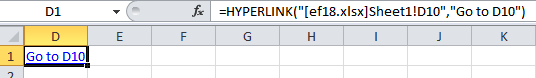
Note how I have to include the file name and the sheet name in the ‘link_location’ argument. It’s a hassle.
But not anymore. The other day I stumbled upon Jerry’s genius use of the # symbol to create a relative reference for the hyperlink.
Now, I know you’re probably thinking why don’t I just use the Insert Hyperlink dialog box and be done with it…well, I could but that is only good if I want one static link.
You see, the advantage for using the HYPERLINK function is that you can build dynamic hyperlinks using functions that reference other cells. Once you build one formula you can copy and paste it to automatically create more, like this:
But first…what’s the magic # all about?
The # symbol works like a relative reference for a hyperlink. So, in the example above instead of having to type out the file name you can just insert #.
Here are some ‘Before’ and ‘After’ examples which illustrate just how handy the # symbol is:
Hyperlink Formula – Go to cell D10 on the Same Sheet
Before magic #:
=HYPERLINK("[ef18.xlsx]Sheet1!D10","Go to D10")
Or with a formula that automatically detects the file and sheet names (this is important if you send the file to other’s who are likely to rename the file and,or change the sheet name):
=HYPERLINK(CONCATENATE("[",MID(CELL("filename"),SEARCH("[",CELL("filename"))+1,LEN(CELL("filename"))-SEARCH("[",CELL("filename"))),"!D10"),"Go to D10")
Ugh. That formula is 150 characters long!
After magic # - the formula is only 30 characters:
=HYPERLINK("#D10","Go to D10")
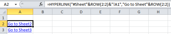
Hyperlink Formula – Go to cell D10 on a Different Sheet
Before magic #:
=HYPERLINK("[ef18.xlsx]Sheet2!D10","Go to Sheet2 D10")
After magic #:
=HYPERLINK("#Sheet2!D10","Go to Sheet2 D10")
Now you can see how great the magic # is, let's look at a clever use for the Hyperlink function.
Dynamic Hyperlink Lookup
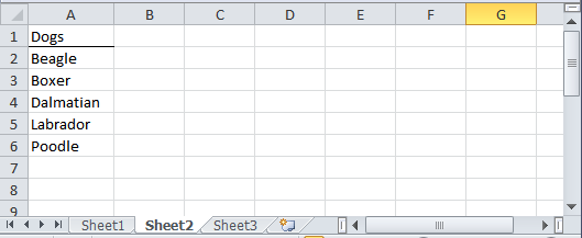
Let’s say on Sheet1 we have a list of dog breeds and we want to insert a hyperlink to take us to the matching breed on Sheet2.
This is Sheet 2:
On Sheet1 (below) we can use the ADDRESS and MATCH functions to find the address (cell reference) of the matching breed on Sheet2 like this:
ADDRESS Function
The ADDRESS function creates a cell reference as text, given specified row and column numbers. The syntax is:
=ADDRESS(row_num, column_num,[abs_num],[a1],[sheet_text])
We only need to complete the row_num, column_num and sheet_text arguments of the ADDRESS function for this formula (the other arguments are optional, hence the square brackets [] ).
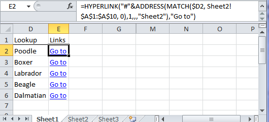
To find the row_num we use the MATCH function to lookup the value in D2 in the range A1:A10 on Sheet2 and return the position i.e. the cell number in the range A1:A10.
Our formula is:
=HYPERLINK("#"&ADDRESS(MATCH($D2,Sheet2!$A$1:$A$10,0),1,,,"Sheet2"),"Go to")
And it evaluates like this:
Step 1 - Poodle is on the 6th row in column A on Sheet2, and since we’re only referencing one column the col_num must be 1, and the sheet name is Sheet2.
=HYPERLINK("#"&ADDRESS(6,1,,,"Sheet2"),"Go to")
Step 2 - The ADDRESS function returns the cell reference which is required for the HYPERLINK formula and rearranges the position of 'Sheet2' in front of the cell reference.
=HYPERLINK("#"&"Sheet2!$A$6","Go to")
Step 3 - The ampersands concatenate all parts of the formula together to give our HYPERLINK function link_location argument.
=HYPERLINK("#Sheet2!$A$6","Go to")
This is just one example of how you can use dynamic hyperlinks. Jerry shows a few more examples on his blog. Plus, you can download a workbook for some clever array formulas that also locate the sheet names, which is handy if you’re working with more than one sheet.
Thanks
Thanks, Jerry for allowing me to share your tip in our Excel Factor series.

Jerry has been using Excel for 20+ years, training and teaching on various Excel Forums for the past 6 years. He is currently one of the Excel Forum Gurus and a Moderator at ExcelForum.com, as well as a registered Software Expert at AskMeHelpDesk.com. He was awarded MVP in Excel by Microsoft in 2010.Jerry Beaucaire is currently the Director of Training, DevStudios America, LLC. He runs a private Excel programming and Consulting business and finds Excel to be "as fun and addicting as Soduko."

Thank you for sharing 🙂
Hi,
I have named ranges on a sheet that contain the names of other sheets in the workbook.
I want to be able to dynamically set the hyperlink to the correct sheet by only referencing the named range. Is this possible? The reason for this, is that the members of the teams will constantly be changing.
Thanks,
Dan.
Hi Daniel,
Check this sample file, there are multiple options. If you can’t make it work, please upload a sample file on our forum to see your data structure, this way we will be able to provide a functional solution.
if sheet is hidden how to use hyperlink function, please help
Hi Bassam,
You can’t go to a hidden sheet via a Hyperlink, sorry. You have to unhide the sheet.
Mynda
Hi Jerry, I am trying to get hyperlinks into the result set from a called vba function. Would you be able to provide guidance on that?
Thank you!
Hi Lesli,
Please post your question on our Excel forum where someone can help you with the VBA code.
Mynda
Buen dia
tengo un problema con la macro vlookup y hyperlink mando a buscar un dato pero no me sale el hipervinculo
Hi Fernanado,
Please post your question and sample Excel file in our Forum so someone can take a look. If you can translate it to English then you’ll probably get a quicker response.
Thanks,
Mynda
Hi,
the post is great!. I have a question that you may know the answer.
I have an excel where in the first tab I have a table with 200 references (200 different numbers), and then I have 1 tab for each of those 200 references (each of the 200 tabs have a different number)
In the first tab I want to create a hyperlink for each invidual tab. how I can use the hyperlink formula to use the reference in the table to access each tab?
thanks
Ivan
Hi Ivan,
Try:
=HYPERLINK("#'"&A2&"'!C10","Go to "&A4&"C10")A4 is the cell with the name of the tab. Copy it down as needed.
Cheers,
Catalin
I have an Excel workbook named “A.xlsx” with a sheet named Sheet1 that contains table data wich contains a date column without duplicates for the date.
I have another Excel workbook named “B.xlsx” with sheet names Sheet1 with different data structure but it contains a date column with duplicates.
I want to make a hyperlink from A.xlsx to B.xlsx that based on the date in each row of A.xlsx & refer to B.xlsx where dates are equal to A.xlsx choosen.
Hi Afif,
Since you have only 2 files, I assume you want to set hyperlinks to cells from B, not to files. Because there are multiple matches in B for the selected date, a hyperlink cannot point to multiple cells, only one of them must be set as the linked cell.
You might want to return a list of matches instead of setting hyperlinks, see this article if is helpful for you: lookup-and-return-multiple-matches
I would use Power Query to return that list, if you feel more confortable using this tool.
If you need more help, please upload a sample file to our forum (create a new topic), we will gladly help you.
Catalin
Hi,
This is great thank you.
How would you create a dynamic hyperlink to take you to a column. I am specifically thinking of looking up a specific date in a long-dated cash flow model – this can create dynamic links to specific events.
Would you use cell –> address –> index/match?
Thanks,
Alex
Hi Alex,
You can use the HYPERLINK function:
=HYPERLINK(“#”&ADDRESS(1,1),”Text to display”)
The above example is set to cell A1: ADDRESS(1,1). First argument of the ADDRESS function is the row number, second argument is the column number. You can replace the number with a function that returns a number: MATCH(SearchValue,A1:Z1,0).
=HYPERLINK(“#”&ADDRESS(1,MATCH(SearchValue,A1:Z1,0)),”Text to display”)
can we get the same hyperlink to the file even the linked file is deleted ?
Hi Sudan,
What do you mean? You will be able to create a hyperlink using the address of a deleted file, but it will not be functional and the reason is obvious. Or I may misunderstood your question… If this is the case, please give us more details on what you are trying to do.
Cheers,
Catalin
Hi there, I am trying to create a hyperlink to PDFs located on our office shared drive.
The pdfs will be named PL_0000001 and so on, and the file name is listed in column A of the excel.
Currently I have to hyperlink each doc individually to the full address with HYPERLINK(\\cc_sys01\Pracsys\22695\PL0000001.pdf, link)
Is it possible do create a function like this, where the document title before the .pdf is populated by the text found in column A?
HYPERLINK(\\cc_sys01\Pracsys\22695\”A1″.pdf, link)
and then copy and paste it down the line to create links for each row?
Hi Warren,
You are close:
=HYPERLINK(“\\cc_sys01\Pracsys\22695\”&A1&”.pdf”, “Link”)
You can copy this down.
Cheers,
Catalin
How can I use a # in a hyperlink to an external file:
link = “test help file.mht#First_Steps”
ThisWorkbook.FollowHyperlink link
Thanks for any wisdom
Hi Lionel,
Try these solutions: hyperlink-to-html-files
Hope it will solve your problem.
Cheers,
Catalin
Catalin – thank you but they don’t work for my purposes. It would appear that this is a problem that MS is overlooking for some reason.
I noticed that your link:
link = “test help file.mht#First_Steps”
is incomplete, you have to provide the full path to that file, like:
link = “C:\Users\Catalin\Desktop\test help file.mht#First_Steps”
Changing the default browser may also help.
Cheers,
Catalin
It works fine without the path as the file is in the current directory. It fails on the internal link #Next_Steps. If I remove the #Next_Steps it opens just fine.
Changing the default browser is not an option as I don’t know what browser my users will have as their default.
Thank you very much – I do appreciate your response.
I meant to change the default browser to another then you can switch back to your usual browser; if it’s a registry problem, this switch will trigger a reset of default registry keys, the change does not have to be permanent.
If you send me the mht file, i can take a look, it works fine on my sample file, maybe the bookmark (anchor) is not valid.
You can use our Help Desk system to upload the file, if you still need assistance 🙂
Catalin
A Really Great Job 🙂
thanks a lot Jerry
I’m using VLOOKUP to fill data in a form. One of my columns of data is HYPERLINKS. VLOOKUP hyperlinks are returning this error. “Cannot open the specified file.”
=HYPERLINK(VLOOKUP(B8,MASTER!A2:BN105,66,0),VLOOKUP(B8,MASTER!A2:BN105,66,0))
Any ideas on how to fix the hyperlink returned by vlookup?
Hi Laurie,
Please upload a sample file , we have to see and analyze your data to understand where is the error comming from.
You can use our Help Desk to upload the file.
Thanks for understanding,
Catalin
Hi,
I have a problem in excel Hyperlink,
i am trying to access a folder named as ‘saju#1’ through hyperlink,
but not yet get solved,
Can any one help me to solve this problem of having “#” symbol in a folder, i dont want to remove/rename the folder.
Hi Saj,
Sorry but I think there is no way to do what you want.
The # symbol is used in hyperlink to link to ‘anchors’ (locations) within a webpage or a document. Specifically with Excel, it uses the # symbol to link to locations in a workbook indicated by a defined name.
Either way, in a hyperlink the # character has a special meaning and when used in a file/folder name you won’t be able to open that file/folder.
Regards
Phil
HI Mynda,
I am an intermediate user in excel and using your website to hone my skills further into excel. I’ve a question with regards to creating links in excel .
Let’s say I am creating an excel sheet whereby I want to put in Column A name of the departments, and on the second column the representative or advisor/s for that department. I want users to be able to click on the name of the advisor, and as soon as they click it leads them to an email in outlook to that person.
Anyhelp in doing this will be greatly appreciated.
Thank You,
Amir
Hi Amir,
You can insert a hyperlink that creates and email in Outlook.
1. Right click in the cell and choose ‘Hyperlink’
2. Enter values for the ‘Text to display’, the ‘E-mail address’ and the ‘Subject’
3. Click OK
Clicking on that hyperlink should now open an email in Outlook (assuming you have Outlook as you default email program.
regards
Phil
Thanks very much Philip-
Hi Amir,
You can use the HYPERLINK function, works beautifully with mailto: applications, you can even add cc or bcc, subject or body to that email. The formula:
=HYPERLINK("mailto:"&C2&"[email protected]&[email protected]&subject=Email To "&B2&", "&A2&" advisor&body=Hi "&B2&",", "Click here to Send Email to "&B2)Can be found in the sample workbook uploaded on our OneDrive folder.
Of course, an alternative is to click on cells from column C that contains email addresses, excel will open automatically a new email message with that email address, but it will not add the other fields like cc, bcc, subject, or body.
Catalin
Thanks Catalin – greatly appreciate your timely response and help.
Regads,
Amir
You’re wellcome Amir 🙂
Looks like you got at least 3 solution for your problem, i answered to you in the same time with Philip 🙂
Cheers,
Catalin
Great post thanks. I was cruising along using a derivative of this code and ran into a challenge. I believe there may be an 85 character limitation bringing the text over to the Outlook mail or so many megabytes to the message. The #VALUE error will end the functionality of the hyperlink. I added “&Left( G13,80)&” to the code below which truncated the cell text, but kept the functionality. Anyone know how to get around the length issue?
=HYPERLINK(“mailto:”&$K$1&”?cc=”&$K$2&”&subject=Narrative Feedback “&B13&”&body=”&G13&””,”Click here to Send Email to MySite”)
Thanks,
Steven
Hi Steven,
The limit is 255 characters, from what i know. And there is no easy way to bypass this limitation, only hyperlinks to web pages can be shortened with a URL shortener via VBA. Or, you can add the hyperlinks via VBA (not working on all excel versions):
ActiveSheet.Hyperlinks.Add Anchor:=Cells(1, “C”), Address:=Cells(1, “A”) & Cells(1, “B”), TextToDisplay:=Cells(1, “B”).Value
Catalin
Thanks. I couldn’t find any other reference pulling in this number of characters, regardless the hyperlink mailto: was great. Thanks again.
You’re wellcome Steven 🙂
Hi.,
Please help to advise..,
Currently I’m using Excel 2010.,
I got the problem for my hyperlink.,
I got more than 1k sheet in my excel.,
Each sheet will link back(using hyperlink) to my main sheet.,
Here my problem arise
When i link back my main sheet, it took me back to cell A1.,
Before.,
When I click link back it will back at my current work for example cell A954.,
Thanks!
Hi,
Can you please upload a sample workbook on our Help Desk?
It will be a lot easier for us to understand the problem and to find a solution.
Thanks,
Catalin
Mynda,
As a follow up to my previous comment, a variation to that request is to have the result from a data validation list be the name of the worksheet in a hyperlink function. For example, if the file name is MyData.xlsm and on the sheet Product in cell A1 the data validation has P012345. P012345 is the name of the sheet I want to go to – cell C1. So if my formula is =HYPERLINK(“[MyData.xlsm]P012345!C1,”Click Here”), how do I insert the result from the data validation drop down of A1 instead of P012345? I tried =HYPERLINK(“[MyData.xlsm]A1!C1,”Click Here”) or =HYPERLINK(“[MyData.xlsm]=A1!C1,”Click Here”) and other variations, but none worked.
Hi Michael,
You can use the INDIRECT function for this:
=HYPERLINK(INDIRECT("[MyData.xlsm]"&A1&"!C1&")Kind regards,
Mynda.
Hi Mynda,
I’ve tried your solution to Michael Rempel’s question, but for some reason it doesn’t work…
I have a different solution. It might be a bit cumbersome (and long…), however it has an advantage: it is a dynamic hyperlink – which means that if Michael wishes to “go to” another sheet name and/or another cell within that sheet – there’s no need for him to make any modifications to the formula!.
Here is my solution to his problem:
If we want the Hyperlink to take us to a specific cell within a specific sheet,
we define the sheetname in A4 and the cell’s address in B4.
We create the hyperlink link (the “goto” address) by concatenating 3 strings:
1)Sheet Name – defined in A4
2) “!”
3) Cell Address – defined in B4
And the full-fledged formula is:
=HYPERLINK(“#”&CONCATENATE(INDIRECT(ADDRESS(4,1)),”!”,INDIRECT(ADDRESS(4,2))),”Go To: Sheet,Cell defined in A4, B4″)
Now, if one wishes to go to a different location, all he has to do is change the target sheet name (in cell A4) and/or the target cell (in cell B4). Using the magic # one doesn’t even need to specify the workbook’s name.
BTW, have you tried my homophones challenge? I wonder if you can find new ones…
Best Regards,
Meni Porat
Hi Meni,
Thanks for sharing your solution 🙂
I have already tried your homophones challenge and all the ones that came to mind were already there 🙁
Kind regards,
Mynda.
Hi Mynda,
I take your disappointment(?) as a compliment. 🙂
Thanks.
🙂 yes, indeed.
Meni,
I was able to get it to work with the following:
=HYPERLINK(“#” & $C1 & “!A1″,”Click Here”)
Thanks,
Michael
Hi Michael,
Nice!
With a slight modification, you can parameterize not only the target sheet name, but also the specific cell within that sheet:
=HYPERLINK(“#” &$C1 & “!” &$A1,”Click Here”)
where the target sheet name is defined in cell C1,
and the target cell is defined in cell A1.
Best Regards,
Meni Porat
Mynda, I hope you can help. I’m trying to create a dynamic link based on the following. In column C I use data validation to pick the description of a part. In column D I use VLOOKUP to pick the Part #. The Part # is the same as the name of another sheet in the workbook (i.e. 030110) with the inventory details of that Part #. I want a dynamic link to cell A1 of that Part # sheet. I am fine with using a helper column (column O). Can you please help?
I often Paste the List of named ranges of a workbook into the workbook for as reference and verification. I used the hashtag tip with hyperlink and indirect functions to create a link to the named range.
Example:
Named range=My_Range covering cells B1:B10
The text “My_Range” is in cell A1
In cell A2, put the formula:
=HYPERLINK(“#indirect(A1)”,”Go to Range”)
When you click A2, it goes to the range My_Range in cells B1:B10. Of course it’s most useful when the range is on another sheet. In my case, I’d copy down the formula for every value in the Paste List. It just saves me from having to click Edit | Goto, in the case of Excel 2003, and scrolling through the long list.
Nice tip. Cheers, Craig 🙂
Thanks again for this tip. It worked for me when the usual hyperlink formula was not working. I use it to save time and brain space in tracking mortgage applications.
Keep up the good work.
Awesome! You Mynda and Jerry simply rock. This site is definitely to going to my Delicious bookmarks right now. Blessings.
🙂 thanks, 6tel.
Hi Mynda. By the way, I finally tried this on this recent weekend, but dynamic hyperlinks in my worksheet do not work after inserting new columns to my sheet… I feel a bit dissapointed because I thought that’s what they’re for… I don’t know what I did wrong… This is the syntaxis I used for one of the links:
=HYPERLINK(“#QK2″,”Facebook · ATH POP”)
It was working fine, till my partner decided to insert some columns in the worksheet where the link was… And it stills points to the cell is supposed to, but I thought it would self-change when new blank columns are added… Like going to the QM2 cell instead of remaining in the same QK2…
Hello 6tel,
Your formula is correct. However, due to the fact the Link Location or “#QK2” is enclosed with Quotation Marks, it means it’s bound to be in the same cell unless the value inside it is manually changed.
It is dynamic in the sense that if the file is sent to a different user and someone changed the file name, all HYPERLINK formulas will still work.
A workaround is to use a formula like this:
=HYPERLINK("#"&ADDRESS(ROW(QK2),COLUMN(QK2)),"friendly name")Now when you insert a row or column it will dynamically update.
Thanks!
Mike
Very good tip.
I think this can be used well for creating index when there are many sheets in the file.
I generally have more than 20 sheets in a file. So now I can create easily the index. There were hyperlink function in excel but that was tedious to use.
Thanks
Cheers, Manish 🙂
Interestingly the use of the # … thanks for the trick Jerry!
I have a suggestion … the last argument of the ADDRESS function is the name of the sheet … so the formula will be:
=HYPERLINK(“#”&ADDRESS(MATCH($D2,Sheet2!$A$1:$A$10,0),1,,,”Sheet2″),”Go to”)
the advantage is for the particular names, for example, a name with spaces (Sheet 2) or a name that contains special characters … the single quote (Sheet’2) … the path is properly written with the addition of characters required
I would also like to tell you that we have written this article a few days ago:
Excel-Hyperlink-to-a-dynamic-range
it is a good alternative and I think that may interest you.
Best regards
r
Thanks, r.
Good point. If the sheet name has a space of special character then your formula works and my original formula (below) breaks 🙁
My original formula:
=HYPERLINK("#"&"Sheet2!"&ADDRESS(MATCH($D2,Sheet2!$A$1:$A$10,0),1),"Go to")I realised that Jerry’s example on his website is the same as yours…I inadvertently changed it. Sorry, Jerry.
Note: I have amended the post above to reflect the better solution that both yourself and Jerry use.
Thanks for your comment 🙂
Mynda.