• Skip to main content
  • Skip to header right navigation
  • Skip to site footer

My Online Training Hub

Learn Dashboards, Excel, Power BI, Power Query, Power Pivot

  • Courses
  • Pricing
    • Free Courses
    • Power BI Course
    • Excel Power Query Course
    • Power Pivot and DAX Course
    • Excel Dashboard Course
    • Excel PivotTable Course – Quick Start
    • Advanced Excel Formulas Course
    • Excel Expert Advanced Excel Training
    • Excel Tables Course
    • Excel, Word, Outlook
    • Financial Modelling Course
    • Excel PivotTable Course
    • Excel for Customer Service Professionals
    • Excel for Operations Management Course
    • Excel for Decision Making Under Uncertainty Course
    • Excel for Finance Course
    • Excel Analysis ToolPak Course
    • Multi-User Pricing
  • Resources
    • Free Downloads
    • Excel Functions Explained
    • Excel Formulas
    • Excel Add-ins
    • IF Function
      • Excel IF Statement Explained
      • Excel IF AND OR Functions
      • IF Formula Builder
    • Time & Dates in Excel
      • Excel Date & Time
      • Calculating Time in Excel
      • Excel Time Calculation Tricks
      • Excel Date and Time Formatting
    • Excel Keyboard Shortcuts
    • Excel Custom Number Format Guide
    • Pivot Tables Guide
    • VLOOKUP Guide
    • ALT Codes
    • Excel VBA & Macros
    • Excel User Forms
    • VBA String Functions
  • Members
    • Login
    • Password Reset
  • Blog
  • Excel Webinars
  • Excel Forum
    • Register as Forum Member

Excel Factor 20 Custom Number Format Disguise

You are here: Home / Excel / Excel Factor 20 Custom Number Format Disguise
Excel Factor 20 Custom Number Format Disguise
October 24, 2012 by Mynda Treacy
This Excel Factor tip was sent in by Marc Joannette of Montreal, Canada.

Words by Mynda Treacy.

Marc's job involves reissuing airline tickets. Part of this process requires a 'reason code' to be selected from a list. So he built a form where you can select a reason from a data validation list and the reason code (number) will be returned, like this:

Excel Custom Number Format with Data Validation

And the good news is it doesn’t use any fancy formulas, just some simple custom number formats and a little Data Validation.

Step 1 Custom Number Format

First Marc set up a list of reason codes to feed the data validation list.

As you can see in the example below each cell contains the reason code description, but if you look in the formula bar you can see the value in the cell is actually the reason code number.

Excel Custom Number Format with Data Validation

To do this Marc entered his reason codes in cells A1:A4, then set up separate custom number formats for each cell which displayed the reason description instead of the actual number value in the cell.

How to Set up a Custom Number Format

  1. To set up a custom number format select the cell you want to format then press CTRL+1 to open the Format Cells dialog box.
  2. On the Number tab select ‘Custom’ from the ‘Category’ list.
  3. In the ‘Type’ field Marc entered his custom number format, which is simply the reason description enclosed in double quotes (see image below).
  4.  

    Excel Custom Number Format

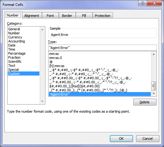
In fact any number that is entered in a cell formatted with the above custom number format will display ‘Agent Error’.

A little about custom number formats:

Number formats can have up to 4 sections of code which are separated by semicolons. Each code section defines the format for positive numbers, negative numbers, zero values and text, in that order.

<POSITIVE>;<NEGATIVE>;<ZERO>;<TEXT>

In Marc’s custom number format he only has one section of code (“Agent Error”), which means that this number format will be applied for all sections of the code.

Now, Custom Number Formats is a topic all on its own, so rather than digress; here is a link where you can read Jon von der Heyden’s comprehensive guide to custom number formats. Click the link later though as I'm not finished explaining Marc's tip... 🙂

Step 2 Data Validation List

Set up the Data Validation list referring to the custom formatted cells A1:A4 (I’ve given them a named range ‘reason_codes’).

  1. Select the cells to which you want to apply the Data Validation List.
  2. On the Data tab of the ribbon select Data Validation
  3.  

    Excel Custom Number Format

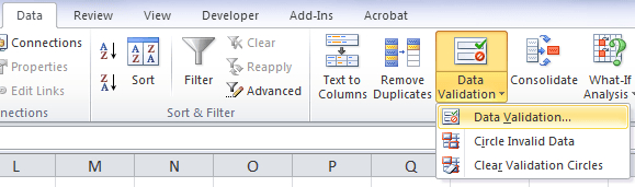
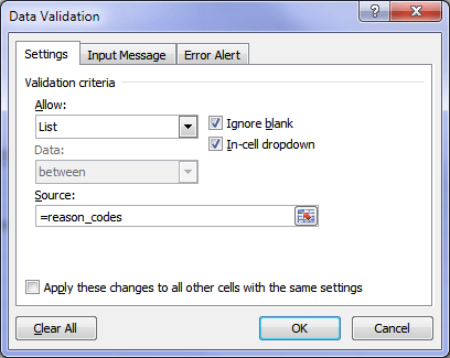
    This will open the Data Validation dialog box below. In the settings tab select ‘List’ from the ‘Allow’ criteria and in the ‘Source’ enter your range or in my case, ‘named range’, and press OK.

    Excel Custom Number Format

Now when you select the cells with data validation you will be able to choose from the exception code descriptions and have the reason code number value returned:

Excel Custom Number Format with Data Validation

The benefit of this approach is that you can use the underlying number value in other formulas that do not handle text, like SUM, AVERAGE, MIN, MAX etc.

Enter your email address below to download the sample workbook.

By submitting your email address you agree that we can email you our Excel newsletter.
Please enter a valid email address.

Download the Excel Workbook. Note: This is a .xlsx file. Please ensure your browser doesn't change the file extension on download.

Thanks for sharing your tip, Marc.

A few words from Marc:

“I am not a programmer but I am a technical person in general (my family would call for help with simple computer installations and formatting, and at work I understand the software and "programmable keys" and I use them to the maximum), but up until last year, I only used Excel for my monthly budget.

Last year, I wanted to do an airline reissue template to assist me in manual airline ticket reissues, (that is the work I do)  ... those PFC taxes are calculated as an amount per departure city, up to four cities, then it's the first 2 cities and the last two cities,  ... it was so hard to do that formula - the first 2 and last 2, or in my case about 16 formulas to get the result needed(version 1)...the final version, has a lot less.

The more I learnt, the more I caught on and enjoyed.

I have found a passion for finding a formula that will do what I want it to do."

Marc

http://excelxfd1048576.wordpress.com/

Vote for Marc

If you’d like to vote for Marc's tip (in X-factor voting style) use the buttons below to Like this on Facebook, Tweet about it on Twitter, +1 it on Google, Share it on LinkedIn, or leave a comment to thank Marc for taking the time to suggest this tip….or all of the above 🙂

Excel Factor 20 Custom Number Format Disguise

More Custom Number Formats Posts

More Data Validation Posts

select multiple items from drop down data validation list

Select Multiple Items from Drop Down (Data Validation) List

Choose multiple items from a data validation (drop down) list and store them all in the same cell. Sample workbook with working VBA.
Searchable Drop Down List in Excel

Searchable Drop Down List in Excel

This searchable drop down list in Excel includes an option for "All" and ignores duplicates. No VBA and no formulas. You won’t believe how easy it is.
selecting multiple items in data validation list

Populating Multiple Cells from Single Data Validation (Drop Down) List

Using a little VBA we can use a single data validation list to select multiple items and populate multiple cells
Automatically Add Items to Data Validation List

Automatically Add Items to Data Validation List

Automatically Add Items to Data Validation List by typing in the new data. Then sort the source list for bonus points
Excel Custom Data Validation

Excel Custom Data Validation to Limit Entries

Excel Custom Data Validation enables you to limit the value or number of entries in a range of cells.
Excel Combo Box KO’s Data Validation

Excel Combo Box KO’s Data Validation

Use an Excel Combo Box as an alternative to Data Validation Lists
Excel Tables as Source for Data Validation Lists

Excel Tables as Source for Data Validation Lists

Excel Factor 19 Dynamic Dependent Data Validation

Excel Factor 19 Dynamic Dependent Data Validation

Excel Data Validation With Dependent Lists

Excel Data Validation With Dependent Lists

excel drop down lists

Excel Drop Down Lists

Excel Drop Down Lists or Data Validation Lists as they're officially known, are a great tool speeding up data entry and ensuring data is entered correctly.

More Excel_Factor Posts

Excel Factor Voting Roundup

Excel Factor Voting Roundup

Excel Factor 21 Hyperlink Triptych

Excel Factor 21 Hyperlink Triptych

Tips and tricks with hyperlinks to make them dynamically update as the selection in the sheet changes. Sample workbook available.
Excel Factor 19 Dynamic Dependent Data Validation

Excel Factor 19 Dynamic Dependent Data Validation

Excel Factor 18 Dynamic Hyperlinks and the Magic Hash

Excel Factor 18 Dynamic Hyperlinks and the Magic Hash

The Excel HYPERLINK function creates links to places inside or outside of your Excel file. I'll show you a shortcut for creating them that few people know.
Excel Factor 17 Lookup and Return Multiple Matches

Excel Factor 17 Lookup and Return Multiple Matches

Excel Factor 16 Dynamic Lookup

Excel Factor 16 Dynamic Lookup

Excel Factor 15 The Lazy Lookup

Excel Factor 15 The Lazy Lookup

Excel Factor 14 Interleave Data from Two Columns into One

Excel Factor 14 Interleave Data from Two Columns into One

Excel Factor 13 Handy Tips & Tricks

Excel Factor 13 Handy Tips & Tricks

Excel Factor 12 Secret EVALUATE Function

Excel Factor 12 Secret EVALUATE Function

More Excel Posts

tips for working in multiple excel files

Hacks for Working in Multiple Excel Files

Awesome tips for navigating, arranging and working in multiple Excel files. Guaranteed to streamline your workflow and increase productivity.
chatgpt for excel

ChatGPT for Excel

Using ChatGPT for Excel can be hit and miss. Learn the best uses for ChatGPT to make your Excel life easier and what to avoid using it for.
excel templates

Where to Find Free Excel Templates

Where to find free Excel templates and how to create your own Excel templates. Using templates saves time and effort.
Easily Remove Password Protection from Excel Files

Easily Remove Excel Password Protection

How to remove Excel password protection when you’ve forgotten the password. Works for sheets, workbooks and read only files.
Import data from a picture to Excel

Import Data from a Picture to Excel

Import data from a picture to Excel. Works with pictures from a file or the clipboard and loads it to the spreadsheet.
excel online

5 Excel Online Features Better than Desktop

5 Excel Online Features Better than Desktop including searchable data validation, track changes, single line ribbon and more.

10 Common Excel Mistakes to Avoid

10 common Excel mistakes to avoid, including merge cells, external links, formatting entire rows/columns and more.
new Excel features

Cool New Features in Excel for Microsoft 365

Cool New Features in Excel for Microsoft 365 including the navigation pane, smooth scroling, unhide multiple sheets and more.
dynamic dependent data validation

Dynamic Dependent Data Validation

Dynamic Dependent Data Validation with dynamic array formulas like FILTER make it quick and easy to set up.
QAT

Excel Quick Access Toolbar

The Excel Quick Access Toolbar is not only a handy for your mouse, but it also enables some super easy keyboard shortcuts.


Category: ExcelTag: Custom Number Formats, Data Validation, Excel_Factor
Previous Post:Excel Factor 19 Dynamic Dependent Data ValidationExcel Factor 19 Dynamic Dependent Data Validation
Next Post:Excel Factor 21 Hyperlink TriptychExcel Factor 21 Hyperlink Triptych

Reader Interactions

Comments

  1. Phil Kowalski

    March 26, 2014 at 6:37 pm

    Hey Mynda,

    just saw this post from the other one about custom number formats. First I though that this does only work with numbers but I found a way around it.

    I had a three letter shortcode which I would have loved to be replaced with its “long name”.

    E. g. AAA should be replaced “My long name”

    The article refers to replacing positive numbers but if you put three semicolons in front of it, the approach works as well for texts. See also Mynda’s post on custom number formats from 03/21/2014.

    Reply
    • Mynda Treacy

      March 26, 2014 at 7:47 pm

      Brilliant! Thanks for sharing, Phil.

      Reply
  2. Raymond

    March 21, 2014 at 9:39 pm

    Hi Mynda,

    As always, awesome little tricks 🙂
    Muchos gracias.

    Gr,
    Raymond

    Reply
    • Mynda Treacy

      March 22, 2014 at 7:17 am

      You’re most welcome, Raymond 🙂 Glad you liked them.

      Reply
  3. Turab

    October 25, 2012 at 8:32 pm

    Can a XL sheet be used as a form on the VB? If so then can we use this concept for creating a Combo Box and selet item from the list of from that box.

    Reply
    • Mynda Treacy

      October 25, 2012 at 9:54 pm

      Hi Turab,

      No, Combo Boxes return a reference number that represents the number of the item in the selected list. i.e. if you select the first item it returns a 1, the second item a 2 and so on.

      However, the Combo Box will display the ‘Source Description’ as opposed to the underlying ‘Source Code’.

      Kind regards,

      Mynda.

      Reply
  4. Andrew Evans

    October 24, 2012 at 5:41 pm

    There is an error in the spreadsheet – it doesn’t explain how you get the number returned instead of the text – and the displaythis named range has the #REF! error against it for both columns. I have liked a lot of the tips sent through but this one has me baffled as the explaination is not so thorough.

    Reply
    • Mynda Treacy

      October 24, 2012 at 6:53 pm

      Hi Andrew,

      Thanks for your comment. The ‘displaythis’ named range is redundant and should not be in the file. I didn’t notice it was still there. As you will see from my explanation I don’t refer to it at all. Sorry for the confusion. I have updated the file now.

      I’m sorry my explanation wasn’t clear enough. Please let me try to explain again how Marc achieved this:

      1. he typed the numbers 10,11,12 and 20 in cells A1:A4. He then selected each cell and set up a custom number format that displayed only the reason code description (see step 1 above for how to do this).

      2. Then give the cells A1:A4 a named range ‘reason_codes’.

      3. Select the cell you want your data validation list in > Data tab of the ribbon > Data Validation > choose List and in the Source field enter =reason_codes

      Your validation list will display the reason code description, but when you select an item from the list it will return and display the reason code number because the cell containing the data validation list isn’t formatted with the custom number format and so it displays the actual value, whereas the data validation list is referencing a range of cells that are formatted with custom number formats to only show the reason code description.

      I hope that fills in the blanks for you. Please let me know if it’s still unclear.

      Kind regards,

      Mynda.

      Reply
  5. jed

    October 24, 2012 at 2:23 pm

    thanks for sharing this.. i might use it in another project. right now, i was looking at the data spread over by daily basis on my monthly list with employees names on the left and the assigned work orders on the right corresponding each day of the month. Some of them are assigned in the same job per day and i need to count the number of employees working there by work orders on daily basis. please help me solve this.. thanks.

    Reply
    • Mynda Treacy

      October 25, 2012 at 9:55 pm

      Hi Jed,

      I’m pleased you’ll find a use for it.

      I’ll speak to you offline about counting the number of employees by work order etc.

      Kind regards,

      Mynda.

      Reply

Leave a Reply Cancel reply

Your email address will not be published. Required fields are marked *

Current ye@r *

Leave this field empty

Sidebar

More results...

Featured Content

  • 10 Common Excel Mistakes to Avoid
  • Top Excel Functions for Data Analysts
  • Secrets to Building Excel Dashboards in Less Than 15 Minutes
  • Pro Excel Formula Writing Tips
  • Hidden Excel Double-Click Shortcuts
  • Top 10 Intermediate Excel Functions
  • 5 Pro Excel Dashboard Design Tips
  • 5 Excel SUM Function Tricks
  • 239 Excel Keyboard Shortcuts

100 Excel Tips and Tricks eBook

Download Free Tips & Tricks

Subscribe to Our Newsletter

Receive weekly tutorials on Excel, Power Query, Power Pivot, Power BI and More.

We respect your email privacy

Guides and Resources

  • Excel Keyboard Shortcuts
  • Excel Functions
  • Excel Formulas
  • Excel Custom Number Formatting
  • ALT Codes
  • Pivot Tables
  • VLOOKUP
  • VBA
  • Excel Userforms
  • Free Downloads

239 Excel Keyboard Shortcuts

Download Free PDF

Free Webinars

Excel Dashboards Webinar

Watch our free webinars and learn to create Interactive Dashboard Reports in Excel or Power BI

Click Here to Watch Now

mynda treacy microsoft mvpHi, I'm Mynda Treacy and I run MOTH with my husband, Phil. Through our blog, webinars, YouTube channel and courses we hope we can help you learn Excel, Power Pivot and DAX, Power Query, Power BI, and Excel Dashboards.

Blog Categories

  • Excel
  • Excel Charts
  • Excel Dashboard
  • Excel Formulas
  • Excel PivotTables
  • Excel Shortcuts
  • Excel VBA
  • General Tips
  • Online Training
  • Outlook
  • Power Apps
  • Power Automate
  • Power BI
  • Power Pivot
  • Power Query
microsoft mvp logo
trustpilot excellent rating
Secured by Sucuri Badge
MyOnlineTrainingHub on YouTube Mynda Treacy on Linked In Mynda Treacy on Instagram Mynda Treacy on Twitter Mynda Treacy on Pinterest MyOnlineTrainingHub on Facebook
 

Company

  • About My Online Training Hub
  • Disclosure Statement
  • Frequently Asked Questions
  • Guarantee
  • Privacy Policy
  • Terms & Conditions
  • Testimonials
  • Become an Affiliate

Support

  • Contact
  • Forum
  • Helpdesk – For Technical Issues

Copyright © 2023 · My Online Training Hub · All Rights Reserved. Microsoft and the Microsoft Office logo are trademarks or registered trademarks of Microsoft Corporation in the United States and/or other countries. Product names, logos, brands, and other trademarks featured or referred to within this website are the property of their respective trademark holders.