Return An Array From A UDF

• Share on Facebook.
• Share on Twitter.
• Share on Google+
• Share on LinkedIn
• Pin It!

This post is going to look at how to return an array from a udf. My last post looked at how to return a range from a UDF and in that, I included a small, bonus function which gave you the interior color of a cell.

I'm going to modify that function so it becomes an array function, or an array formula as they are also known. Specifically it will become a multi-cell array function as it will return multiple values into multiple cells.

What is an Array?

An array is just a list of values, e.g. 1, 2, 3, 4, 5 is an array with 5 values, or elements

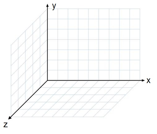
That was an example of a one dimensional array. Think of one dimension representing values along a straight line, like the x-axis on a chart.

A two dimensional array holds values that can be used to represent something that requires two things to identify it, e.g. the x and y co-ordinates on a chart, the squares on a chess board, or even the cells on your worksheet (A1, etc).

Three dimensional arrays contain three lists of values used to identify something (the xyz co-ordinates) perhaps the latitude, longitude and height above sea level of a point on the Earth's surface.

You can have more dimensions of course if you need them, but for my example we're sticking with just one.

Returning Arrays of Different Sizes

In order to process an unknown number of values, we need to work out how many values are passed into our function and then allocate the appropriate amount of storage in an array.

Initially we allocate an unknown amount of storage space for the array named Result():

    Dim Result() As Variant

Once the function is called we can work out how many cells are in the range we're passing into the function. We can do this by using Application.Caller which gives us a Range object, as long as our function is called from a cell. This range is the range of cells passed into the function.

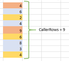
We can work out how many cells in the range and whether we're passing a row or a column into the function

    With Application.Caller
        CallerRows = .Rows.Count
        CallerCols = .Columns.Count
    End With

If CallerRows > 1 then a column is being passed into the function.

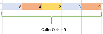
If CallerCols > 1 then a row is being passed into the function.

The number of cells in the range is CallerRows * CallerCols, so we redimension the array to hold a value for each of those cells.

    'ReDimension the array to fit all the elements (cells)
    ReDim Result(1 To CallerRows * CallerCols)

If we pass in a range containing 6 cells, then our result will contain 6 values. Remember that this function is only dealing with one dimensional arrays, that is, values either in a row or a column.

If we pass in a range containing 10 cells, but allocate less than 10 cells for the result, we'll get #VALUE! errors.

If we pass in 6 cells, and allocate more than 6 cells for the result, cells 7 onwards will be filled with 0.

How you choose to deal with this is up to. You can write your own error handling, or just let Excel deal with it.

Don't Forget

This is an array formula, so when you enter it you must use CTRL+SHIFT+ENTER. That is, hold down CTRL and SHIFT, then press ENTER.

Fixed Sized Arrays

If you know the number of elements in your array will be fixed you can specify this and not worry about working it out when the function is called, For example, here's a 10 element array:

Dim myResult(1 To 10) As Variant

But passing in a range with more or less than 10 elements could easily break your function.

Array Orientation

By default a function will return an array as a row. If you want the results to go into a column, you need to transpose the array

    'Transpose the result if returning to a column
    If CallerRows > 1 Then
    
        GetColor = Application.Transpose(Result)
        
    Else
    
        GetColor = Result
    
    End If

Download the Workbook

Here's a link to download a workbook with sample code and examples.

Please Share

If you liked this please click the buttons below to share.