• Skip to main content
  • Skip to header right navigation
  • Skip to site footer

My Online Training Hub

Learn Dashboards, Excel, Power BI, Power Query, Power Pivot

  • Courses
  • Pricing
    • Free Courses
    • Power BI Course
    • Excel Power Query Course
    • Power Pivot and DAX Course
    • Excel Dashboard Course
    • Excel PivotTable Course – Quick Start
    • Advanced Excel Formulas Course
    • Excel Expert Advanced Excel Training
    • Excel Tables Course
    • Excel, Word, Outlook
    • Financial Modelling Course
    • Excel PivotTable Course
    • Excel for Customer Service Professionals
    • Excel for Operations Management Course
    • Excel for Decision Making Under Uncertainty Course
    • Excel for Finance Course
    • Excel Analysis ToolPak Course
    • Multi-User Pricing
  • Resources
    • Free Downloads
    • Excel Functions Explained
    • Excel Formulas
    • Excel Add-ins
    • IF Function
      • Excel IF Statement Explained
      • Excel IF AND OR Functions
      • IF Formula Builder
    • Time & Dates in Excel
      • Excel Date & Time
      • Calculating Time in Excel
      • Excel Time Calculation Tricks
      • Excel Date and Time Formatting
    • Excel Keyboard Shortcuts
    • Excel Custom Number Format Guide
    • Pivot Tables Guide
    • VLOOKUP Guide
    • ALT Codes
    • Excel VBA & Macros
    • Excel User Forms
    • VBA String Functions
  • Members
    • Login
    • Password Reset
  • Blog
  • Excel Webinars
  • Excel Forum
    • Register as Forum Member

Excel Conditional Formatting Highlight Matches in List

You are here: Home / Excel / Excel Conditional Formatting Highlight Matches in List
February 22, 2017 by Mynda Treacy

In this tutorial we’re going to look at how we can use Excel Conditional Formatting to highlight rows in a table where a field matches any item in a list.

Let’s look at an example, below is our table of data:

table of data

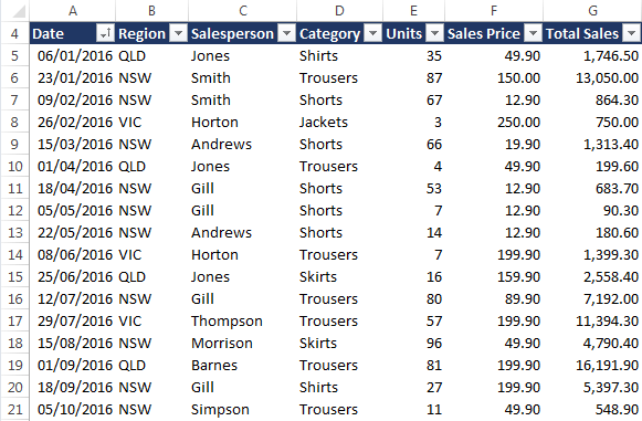
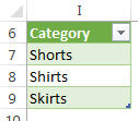
And we want to highlight the rows that contain any of the categories in this Table:
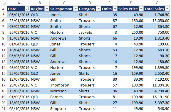
highlight rows

Like so:

named range list

Note: My list is in an Excel Table in cells I7:I9 and I’ve given it the Named Range: List. We’ll be using this name in the Conditional Formatting formula.

Download the Excel File

Enter your email address below to download the sample workbook.

By submitting your email address you agree that we can email you our Excel newsletter.
Please enter a valid email address.

Download the Excel Workbook. Note: This is a .xlsx file please ensure your browser doesn't change the file extension on download.

Setup Conditional Formatting

Step 1: To set up the Conditional Formatting we first select the Table cells we want to highlight, in my case A5:G47.

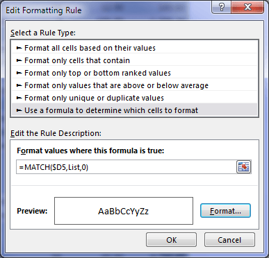
Step 2: Home tab > Conditional Formatting > New Rule > select ‘Use a formula to determine which cells to format’ from the Rule Type list.

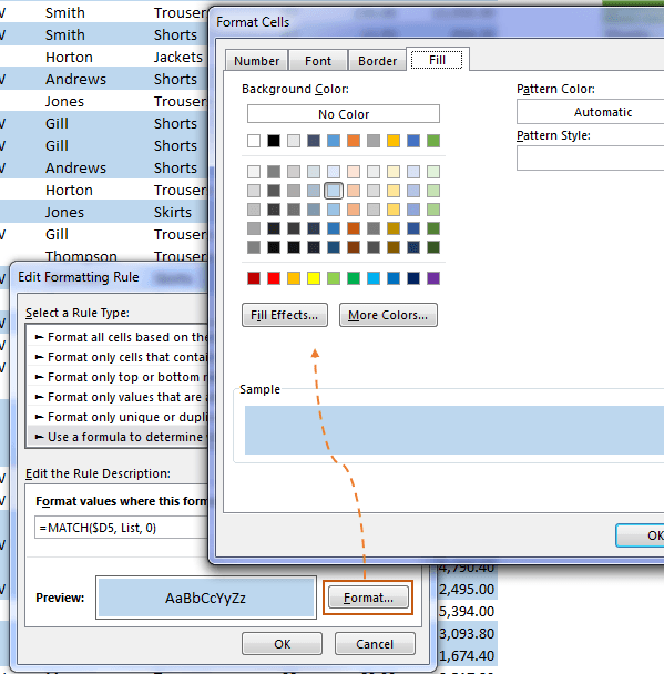
Step 3: Insert the formula

=MATCH($D5,List,0)

In the dialog box as shown below:

dialog box

Now if you remember my post from a couple of weeks ago with a similar example you’ll recall that I said Conditional Formatting formulas must always evaluate to TRUE or FALSE, or their numeric equivalents of 1 and 0.

And if you’re familiar with the MATCH Function you’ll know that it returns the position of a value in a list, and in this example that could be anything between 1 and 3. So you might be wondering how that MATCH formula works in Conditional Formatting.

Taking the formula above, it evaluates like so:

=MATCH($D5, List, 0)
=MATCH("Shirts", {"Shorts";"Shirts";"Skirts"}, 0)
=2

i.e. Shirts is the second item in the ‘List’.

So, the formula isn’t returning TRUE or FALSE, or their numeric equivalent of 1 and 0, yet the format is still applied. What?!

I discovered through experimenting that the conditional format will be applied as long as any (positive or negative) value other than zero is returned by the formula.

That means we could also use this formula to achieve the same results:

=COUNTIF(List, $D5)

Click here for a more thorough understanding of how Conditional Formatting formulas work.

Step 4: Click the ‘Format’ button in the dialog box above and set your format:

set format

Thanks

A big thank you to Cliff Beacham for sharing his 'Excel Conditional Formatting Highlight Matches in List' tip and for teaching me something new.

Cliff has an Excel book coming out soon. Keep your eye out on Amazon for it.

More Excel Posts

excel check boxes

Interactive Excel Check Boxes

Excel check boxes are interactive elements you can link to formulas, charts, conditional formatting and more.
tips for working in multiple excel files

Hacks for Working in Multiple Excel Files

Awesome tips for navigating, arranging and working in multiple Excel files. Guaranteed to streamline your workflow and increase productivity.
chatgpt for excel

ChatGPT for Excel

Using ChatGPT for Excel can be hit and miss. Learn the best uses for ChatGPT to make your Excel life easier and what to avoid using it for.
excel templates

Where to Find Free Excel Templates

Where to find free Excel templates and how to create your own Excel templates. Using templates saves time and effort.
Easily Remove Password Protection from Excel Files

Easily Remove Excel Password Protection

How to remove Excel password protection when you’ve forgotten the password. Works for sheets, workbooks and read only files.
Import data from a picture to Excel

Import Data from a Picture to Excel

Import data from a picture to Excel. Works with pictures from a file or the clipboard and loads it to the spreadsheet.
excel online

5 Excel Online Features Better than Desktop

5 Excel Online Features Better than Desktop including searchable data validation, track changes, single line ribbon and more.

10 Common Excel Mistakes to Avoid

10 common Excel mistakes to avoid, including merge cells, external links, formatting entire rows/columns and more.
new Excel features

Cool New Features in Excel for Microsoft 365

Cool New Features in Excel for Microsoft 365 including the navigation pane, smooth scroling, unhide multiple sheets and more.
dynamic dependent data validation

Dynamic Dependent Data Validation

Dynamic Dependent Data Validation with dynamic array formulas like FILTER make it quick and easy to set up.


Category: Excel
Previous Post:Excel Custom Number Format Guide
Next Post:Power Query Unpivot

Reader Interactions

Comments

  1. lex

    May 8, 2021 at 4:00 am

    Were you able to apply this to your whole table? Or did you have to duplicate the condition for every row?
    Thanks!

    Reply
    • lex

      May 8, 2021 at 4:05 am

      Please ignore my question- I figured it out. I had my first cell locked! Thanks again for this post, it helped a lot!

      Reply
  2. Mylene

    September 17, 2020 at 3:05 am

    This is great, it works! I have a question and I can’t find the answer. Instead of exact “match”, I would like to highlight cells which “contains” the words in my list. Do you know how to do?

    Reply
    • Philip Treacy

      September 17, 2020 at 9:02 am

      Hi Mylene,

      If you mean you have a list of substrings like :

      Sh
      Sk
      Ja

      and you want to check if these substrings appear within other strings you can change the CF formula rule to

      =SUM(IFERROR(SEARCH(List,D5),0))

      If that doesn’t work, please start a topic on our forum and attach your workbook.

      Regards

      Phil

      Reply
  3. Ryan

    September 12, 2018 at 2:31 pm

    I attempted this with the cell value named range in column A and the column to match against in column B. It worked for most values, but was not accurate in every case. For instance, A cell value of “0011I00000Op6ye” in columns A AND B were not highlighted by the conditional formatting.

    Any thoughts….perhaps on how to make it case sensitive?

    Reply
    • Mynda Treacy

      September 12, 2018 at 7:28 pm

      Hi Ryan,

      Can you please post your question and sample Excel file on our forum so we can see how it is constructed and troubleshoot from there.

      Mynda

      Reply
  4. Jonathan Cooper

    February 23, 2017 at 11:33 pm

    If you use an IF statement and in the first argument you refer to is a positive or negative number then the formula will evaluate to TRUE (e.g., =If(1,TRUE,FALSE). A zero or empty cell will result in FALSE (e.g. =If(0,TRUE,FALSE). This is what is happening in the conditional formatting formula.

    I read this somewhere else a long time ago but I don’t remember where.

    Reply
    • Mynda Treacy

      February 24, 2017 at 7:07 am

      Nice, thanks for sharing, Jonathan.

      Mynda

      Reply
  5. jim

    February 23, 2017 at 9:35 pm

    Similarly, the condition for an IF formula can evaluate to any-number-but-zero for the TRUE option to be triggered
    and ehan, I feel you pain, but all you need to do is define a suitably-named range to refer to your table column and it all works (like what Mynda did)

    Reply
  6. Mrefy

    February 23, 2017 at 7:09 pm

    Gents , its not working with me as I followed this step and its highlight all the cells from A5:G47

    Reply
    • Mynda Treacy

      February 23, 2017 at 9:48 pm

      Hi Mrefy,

      I suspect you entered something not quite right. Please double check your formula etc. If you don’t find the problem please post your file and question in our Excel Forum so we can help you.

      Mynda

      Reply
  7. Sunny Kow

    February 23, 2017 at 5:10 pm

    Hi Mynda
    From your example 1 in your workbook,if you use MATCH you need to press CTRL+ALT+F9 before the formatting updates. If you use COUNTIF it automatically update. This seems odd as example 2 works fine without CTRL+ALT+F9.

    Sunny

    Reply
    • Mynda Treacy

      February 23, 2017 at 9:45 pm

      Hi Sunny,

      That’s really odd. I recall testing the first sheet example by changing an item in the list and it worked fine. I was playing around with which categories to use to get the best results for the examples. In fact, if you edit the conditonal formatting rule, but don’t change anything it starts working again! Odd.

      Mynda

      Reply
      • SunnyKow

        February 24, 2017 at 10:12 am

        Hi Mynda
        If you edit the CF, it will work at that point of time. If you save, close and then reopen the file, the CF will not work again when you change the categories.

        Reply
        • Mynda Treacy

          February 24, 2017 at 10:25 am

          It’s the named range not refreshing. If you just reference the cells in the Conditonal Formatting rule it updates immediately. This is why the COUNTIF version works, it doesn’t reference a named range.

          Reply
  8. ehans

    February 23, 2017 at 6:34 am

    It is frustrating that Conditional Formatting doesn’t recognize table references, so you cannot replace =$D6 in your formula with =Table2[@Category], not unless there is some strange syntax I have yet to stumble upon.

    For me, I’d much rather say this conditional format applies to Table2 instead of $A$5:$H$47. Same with columns. Applying a format to =Table2[Sales Price] makes more sense to me than $F$5:$F$47

    Reply
    • Jonathan Cooper

      February 23, 2017 at 11:23 pm

      =MATCH($d5,INDIRECT(“Table2[Sales Price]”),0)

      Reply

Leave a Reply Cancel reply

Your email address will not be published. Required fields are marked *

Current ye@r *

Leave this field empty

Sidebar

More results...

Featured Content

  • 10 Common Excel Mistakes to Avoid
  • Top Excel Functions for Data Analysts
  • Secrets to Building Excel Dashboards in Less Than 15 Minutes
  • Pro Excel Formula Writing Tips
  • Hidden Excel Double-Click Shortcuts
  • Top 10 Intermediate Excel Functions
  • 5 Pro Excel Dashboard Design Tips
  • 5 Excel SUM Function Tricks
  • 239 Excel Keyboard Shortcuts

100 Excel Tips and Tricks eBook

Download Free Tips & Tricks

Subscribe to Our Newsletter

Receive weekly tutorials on Excel, Power Query, Power Pivot, Power BI and More.

We respect your email privacy

Guides and Resources

  • Excel Keyboard Shortcuts
  • Excel Functions
  • Excel Formulas
  • Excel Custom Number Formatting
  • ALT Codes
  • Pivot Tables
  • VLOOKUP
  • VBA
  • Excel Userforms
  • Free Downloads

239 Excel Keyboard Shortcuts

Download Free PDF

Free Webinars

Excel Dashboards Webinar

Watch our free webinars and learn to create Interactive Dashboard Reports in Excel or Power BI

Click Here to Watch Now

mynda treacy microsoft mvpHi, I'm Mynda Treacy and I run MOTH with my husband, Phil. Through our blog, webinars, YouTube channel and courses we hope we can help you learn Excel, Power Pivot and DAX, Power Query, Power BI, and Excel Dashboards.

Blog Categories

  • Excel
  • Excel Charts
  • Excel Dashboard
  • Excel Formulas
  • Excel PivotTables
  • Excel Shortcuts
  • Excel VBA
  • General Tips
  • Online Training
  • Outlook
  • Power Apps
  • Power Automate
  • Power BI
  • Power Pivot
  • Power Query
microsoft mvp logo
trustpilot excellent rating
Secured by Sucuri Badge
MyOnlineTrainingHub on YouTube Mynda Treacy on Linked In Mynda Treacy on Instagram Mynda Treacy on Twitter Mynda Treacy on Pinterest MyOnlineTrainingHub on Facebook
 

Company

  • About My Online Training Hub
  • Disclosure Statement
  • Frequently Asked Questions
  • Guarantee
  • Privacy Policy
  • Terms & Conditions
  • Testimonials
  • Become an Affiliate

Support

  • Contact
  • Forum
  • Helpdesk – For Technical Issues

Copyright © 2023 · My Online Training Hub · All Rights Reserved. Microsoft and the Microsoft Office logo are trademarks or registered trademarks of Microsoft Corporation in the United States and/or other countries. Product names, logos, brands, and other trademarks featured or referred to within this website are the property of their respective trademark holders.