Power Query’s Unpivot tool allows us to fix one of the most common mistakes (many) Excel users make when capturing data in Excel, and that is to use the wrong layout.
You see they tend to jump into a report format, or they might put it in a format that makes it easy for someone to input the data. The problem with this is it makes it very difficult to then use the built-in tools available, tools like PivotTables and formulas.
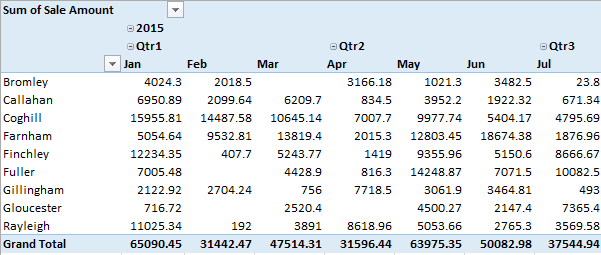
Here’s an example of the wrong layout (don’t be fooled by it’s neat and tidy appearance, it’s evil):
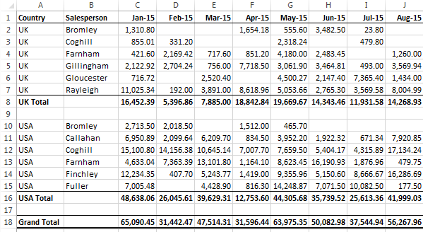
“What’s wrong with this layout”, I hear you say. Well this layout is already Pivoted, in other words this layout is something a PivotTable can produce in seconds. It’s the end result, as opposed to the way you should capture data. Ok, maybe ‘evil’ is a bit harsh, but it’s going to cause you a lot of pain and anguish.
Here’s an example, let’s say you send this report to your boss. Then five minutes later she comes back and says “that report is great, but can you also show me the data grouped by Salesperson by quarter …. Oh, and I need it in 10 minutes for a meeting”.
Right about now you agree with me that this layout is evil. You’ll be lucky to turn this around in ten minutes.
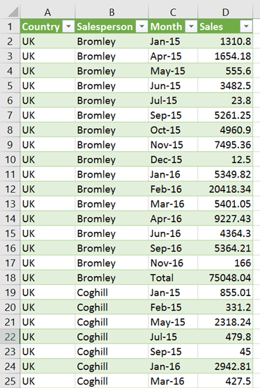
Hold up, before you panic let’s look at a different scenario. What if you had your data in the ideal tabular format like this:
In less than 2 minutes you could create both of your reports from this perfect tabular data using PivotTables. Here they are:
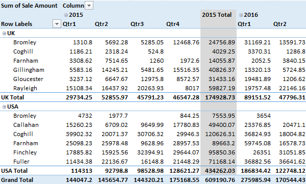
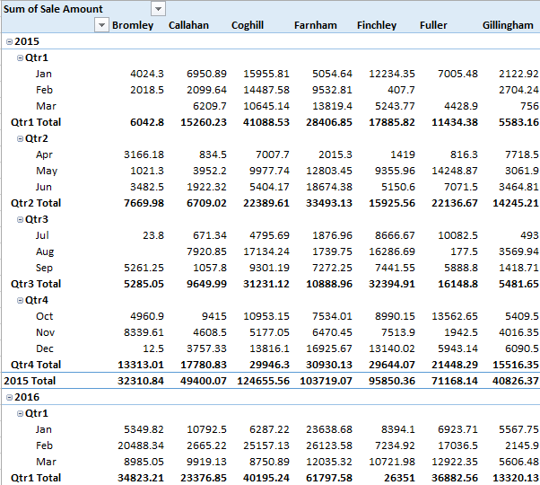
Oops, boss said she wants Salesperson in the rows and periods in the columns. No problem, you can just drag and drop the fields in the PivotTable field list to switch them around. A few seconds later and here it is:
Now, I’m not going to continue with my rant about the right layout for your data, I do that here. Instead I want to show you how you can use Power Query to easily unpivot your data so that it’s in a nice, friendly tabular layout.
Download the Workbook
Enter your email address below to download the sample workbook.
Power Query Unpivot
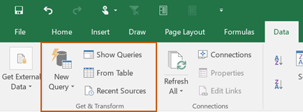
Note: Power Query is available for Excel 2010 onwards. Excel 2010 and 2013 users see system specifications and download it here. For Excel 2016 users, Power Query is already available from the Data tab in the Get & Transform group:
Unpivoting data using Power Query is easy.
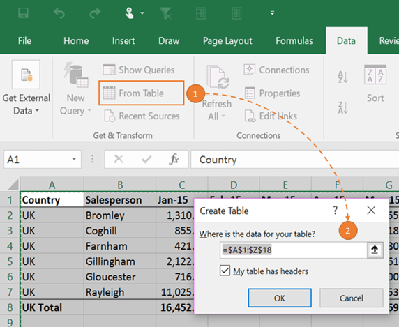
Step 1: Select your data, in my case it’s in cells A1:Z18
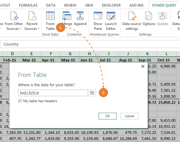
Step 2: Excel 2010 and 2013; on the Power Query tab > From Table. Make sure the range is correct and check the box ‘My table has headers’ (assuming yours does too):
Step 2: Excel 2016; Data tab > From Table:
This will open the Query Editor.
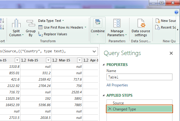
Tip Before moving on, it's a good idea to remove the automatically inserted 'Changed Type' step as this can sometimes cause problems later on. Just click the 'X' to remove it before moving on to Step 3.
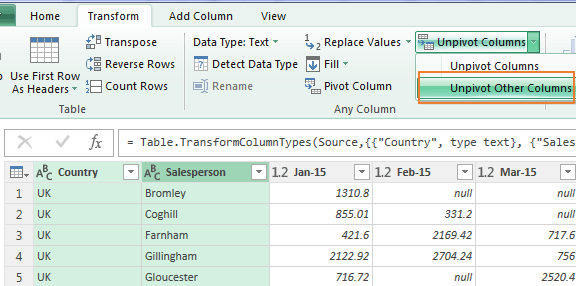
Step 3: In the Power Query editor, which is the same in all versions of Excel, we want to unpivot the columns that contain values. Since we only have a couple of columns that don’t need unpivoting I’ll select them (hold down CTRL and click the Country and Salesperson columns) > Transform tab > Unpivot Columns > Unpivot Other Columns:
It should look like this with the column headers now in the ‘Attribute’ column and the Sales Amounts in a ‘Value’ column:
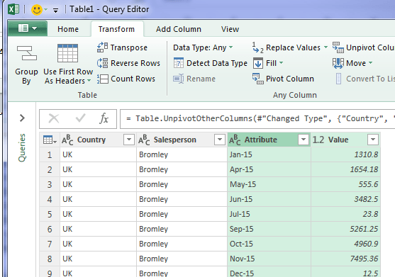
Tip: if you expect to add new columns to your source data, for example figures for a new month, then choosing ‘Unpivot Other Columns’ will ensure any new columns are automatically included when you refresh the query.
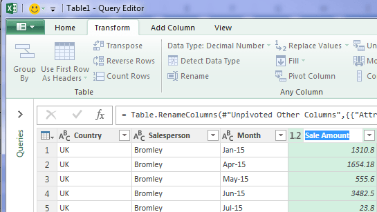
Step 4: Double click the ‘Attribute’ and ‘Value’ column headers and enter more appropriate names:
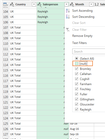
Step 5: If you scroll down you’ll see we have the Total rows still in the data. We can use the filter button on the Salesperson column to filter out all rows that contain ‘null’, which is the equivalent of a blank cell:
The great thing about Power Query is it’s a bit like a Macro recorder in that it records each step as you go. We can see them in the ‘Applied Steps’ list on the right-hand side of the query editor:
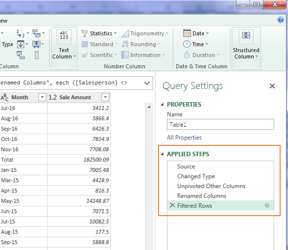
This means that if we update the source data with figures for a new month we can simply click the ‘Refresh’ button on the Data tab and Power Query will get the new data and run it through all the steps without us having to make any changes.
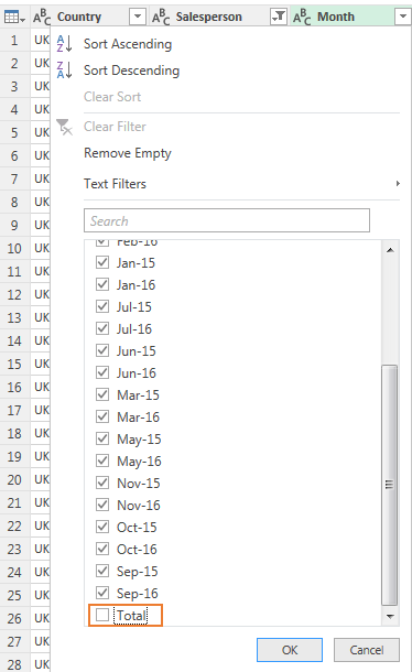
Step 6: We also have a total row in the month column that needs filtering out, so just like the previous step; select the filter button on the Month column > scroll to the bottom and deselect ‘Total’:
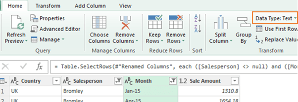
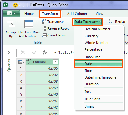
Step 7: It’s always best practice to ensure dates are stored in the correct format in Excel. We can see that the Month column has the Data Type: Text, which will not play nice with PivotTables or formulas.
We can tell this from the Home tab > Data Type is ‘Text’ and the indicator on the column header is ‘ABC’, which means Text:
To fix this, select the ‘Month’ column > Home tab > change the Data Type to ‘Date’:
Note: if you want to practice this using my sample workbook and your date format is mm/dd/yyyy, then you need to change the date type using the Locale. To do this right-click the Month column > Change Type > Using Locale > Data Type: Date and Locale: English (Australia).
Now the Month column has the calendar icon in the header, the dates look like real dates and they’re right aligned:
![]()
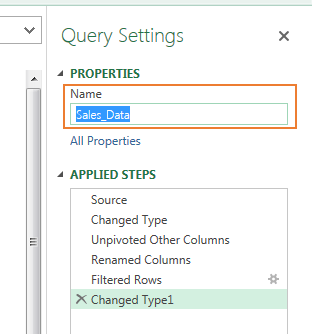
Step 8: Name the query; let’s give the query a meaningful name, rather than the default table name.
This will help us identify the data more easily when we reference it in our PivotTables and formulas. Simply type over the name in the Properties Name field in the right-hand side of the query editor:
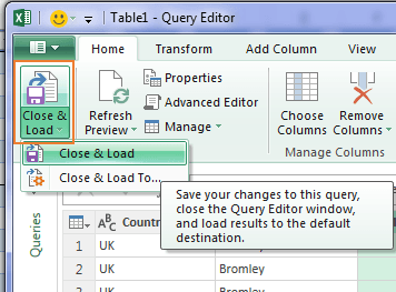
Step 9: Close & Load: we’re ready to load the data into Excel. Home tab > Close & Load:
This will put your data in an Excel Table called ‘Sales_Data’ in a new worksheet in your file, and the Workbook Queries pane will open on the right:
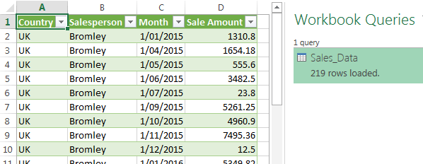
Now you’re ready to analyse and summarise your perfect tabular data with PivotTables, or formulas to your heart’s content.
More Power Query
Click here for more Power Query tutorials.
And if you want to get up to speed quickly please check out my Power Query course.

Mynda, if you are talking about data coming from a database you are correct. If you are talking about creating say a business plan for 3 years by month in Excel, there is absolutely no way any end user would enter data in the “IT friendly” format best suited to Power BI.
You and I both know the time series user friendly years by monthly periods would be used in almost EVERY spreadsheet of this type. That doesn’t negate the need to transform this using powerquery to get the dimensionality required for your Pivot Table examples, but the whole industry around Power BI seems to either negate or ignore this fundamental issue with transforming financial spreadsheets into exciting Pivot Table / Power BI models. I believe this is the biggest barrier at the moment, as almost EVERY Power BI model example shown by the experts just assumes the data arrives in this Power BI optimised format. After 30 years in BI, I can assure you it doesn’t. My rant now over. Would love you to address this practical issue and would be prepared to work with you, if you did.
Hi Paul,
Back when I did budgeting in Excel we had a user friendly front end and then a series of complex formulas that converted the data into the ideal tabular format so we could summarise and analyse it. Nowadays I could use Power Query to convert the data to a tabular format more easily and with less room for error. And while the front end was user friendly, it still met good data layout practices where we didn’t used merged cells or headers spread over multiple rows etc.
I agree, sometimes a user friendly layout is required, but a lot of the time it isn’t. There are plenty of Excel files that are created in the wrong format when they could have used the ideal tabular layout. I saw one just today; they had 16 Tables instead of one. They had the right idea, but they’d unnecessarily split the data into multiple tables. It happens all the time.
“…almost EVERY Power BI model example shown by the experts just assumes the data arrives in this Power BI optimised format” on the contrary, Power Query was developed because data rarely comes in the desired format. With Power Query we can easily fix the data so it’s ready for the Power BI/Power Pivot model. Sure, many companies already have their data in a database that stores it in the right format, and Power BI can connect to that data too, but for users who get their data form Excel spreadsheets where it’s stored in a less than ideal format, Power Query can help.
Mynda
Do you have recommendations are courses on how to tabularize reports and especially if they come from a pdf file?
Hi Marc,
In this tutorial I run through how to convert common report layouts into tabular data. Unfortunately, we don’t have the ability to get data from a PDF with Power Query…yet.
Mynda
Great article Mynda. And I don’t think you are ranting : you absolutely right about the way of the report is laid out ( pivoted) . Many people don’t think about data: they just create outputs in excel and then when they want to analyze the data, they have a hard time changing the data quickly and then excel cannot help you. I always lay my data in tabular form just in case, I need to perform a deep analysis .
Now that I am talking power query: I have a list of words in Spanish that I want to transform using locale: I have words that have the tilde and I want to take the tilde out: Example I have the word acción and I want to change it to accion . Another word is evaluación and I wan to change it to evaluacion. I was trying to play with the locale function in PQ to see if I can change the locale from Spanish to English but I cannot get it to work.My list is 150 rows. Any suggestions on how to change /replace the ‘ . Thanks Again. I am great fan of your blogs and your videos.
Hi Luis,
Great to hear you already use Tabular layouts 🙂
In regards to converting your language, you can’t use Locale for this. You’d have to use Replace text. If you have a lot of different letters with accents you could use this technique.
Mynda
Thanks Mynda,
I love this – and well explained as usual thank you!
This has helped me get some data into Power BI much quicker than I thought possible.
Only problem now is that I have data in many different number formats (percentages, dollars etc) so when I pull them into Power BI everything has the same format…
Any suggestions on how to manage that?
Thanks again
Hi Vaughan,
Great to hear you’re embracing Power Query 🙂
But Power Query is not the place to format the data style/appearance. You can do that in Power BI in the modeling tab.
Mynda
Mynda
Excellent article and sample Excel data for use with Power Query. I’ve never used this before and it’s really useful to learn more about. Thanks very much Mynda!
Thanks, James! Glad you found it helpful.
Great article. It sent me on quite a journey to your other rant, and I also discovered the PivotTable and PivotChart Wizard, best used for those who stubbornly put their data into separate tabbed worksheets by week, month or quarter (arrrrgh!).
You’ve heard of separation of Church and State…. well I call this separation of Data and Presentation. Don’t confuse the two!
🙂 love it, Renny!