A while ago I wrote about to how perform the equivalent of an Excel exact match VLOOKUP formula with Power Query which, by the way, is dead easy. Ever since then I’ve been asked to explain how to do a Power Query approximate match VLOOKUP formula. So, here it is. It requires a few more steps. Nothing too difficult though, I promise.
Watch the Video

Download Workbook
Enter your email address below to download the sample workbook.
Power Query Approximate Match VLOOKUP Written Instructions
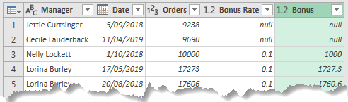
First let’s look at what it means to do an approximate match VLOOKUP. Taking the Orders Table below I want to apply a bonus for each row based on the Order Value bands in the blue ‘lookup table’:
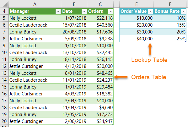
The Order Value in the Bonus table represents the minimum order amount for the corresponding bonus rate e.g. The order on row 8 will not receive a bonus because it’s below the minimum order value of $10,000. And the order on row 7 will attract a 10% bonus because it’s above $10,000 and below the next band of $20,000.
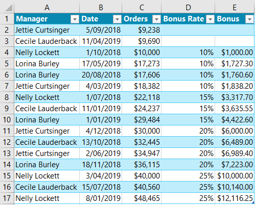
Using VLOOKUP I’d write the formula like so with ‘TRUE’ as the final argument:
=VLOOKUP(C5,$E$5:$F$8,2,TRUE)
The end result looks like this:
Let’s look at how to achieve the approximate match VLOOKUP with Power Query.
Power Query Approximate Match VLOOKUP
Step 1: Load both the Order Table and Bonus Rates Table to Power Query. In Excel 2016 onward – Data tab > From Table/Range. In Excel 2013 and earlier – Power Query tab > From Table/Range:
Note: If you don’t see the Power Query tab in Excel 2010 or 2013 you can download it here.
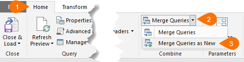
Step 2: Merge the Tables; Home Tab > Merge Queries > As New
This opens the Merge dialog box where you select the two tables from the drop-down lists, then click on the column from each table that the lookup should be performed on. On this case it’s the Orders column from the Orders table and the Order Value column from the BonusRates table:
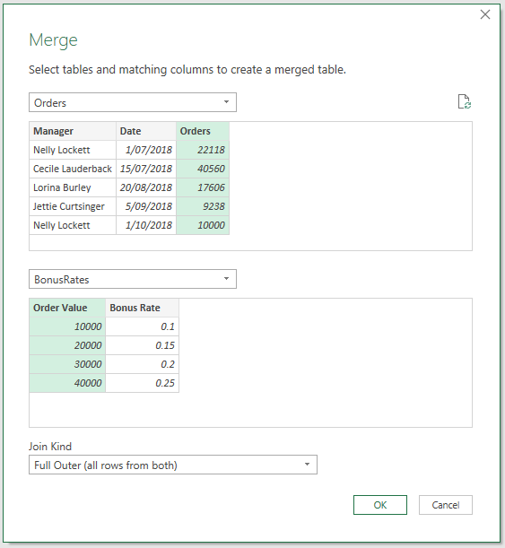
You can see the selected columns highlighted in green. Be sure to choose ‘Full Outer’ in the Join Kind drop-down list at the bottom of the Merge dialog box.
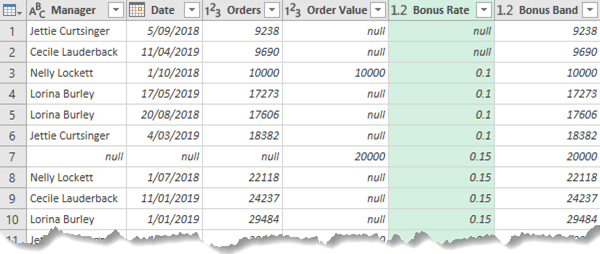
Step 3: Expand the BonusRates table by clicking on the double headed arrow on the column header:
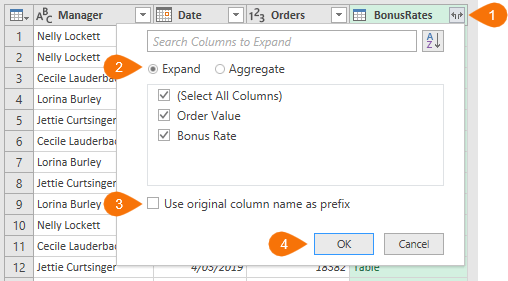
Select ‘Expand’ and deselect ‘Use original column name as prefix' as we don’t need it. It should look like this:
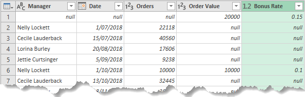
Notice the first row contains null values for Manager, Date and Orders. This is because we don’t have any order values that match the BonusRate Order Value of $20,000. That’s ok. You’ll see why soon.
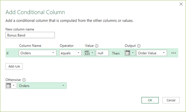
Step 4: Add a Conditional Column that pulls in the value from the Orders column or if null, then the Order Value from the Bonus Rate table.
Add Column tab > Conditional Column. Note: in the Output and Otherwise fields select the Table from the drop-down to the left. This will enable you to select the table name from the list.
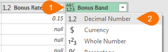
Step 5: Change the data type for the Bonus Band column to decimal number. Click on ABC123 in the column header > Select 1.2 Decimal Number from the list:
Step 6: Sort the Bonus Band column; Select the Bonus Band column header > Home tab > Sort A to Z.
Step 7: Fill down the Bonus Rate; Select the Bonus Rate Column > Transform tab > Fill > Down. It should look like this:
Step 8: Now you can delete the Bonus Band and Order Value columns as they’ve done their job. Select the column headers and press the Delete key.
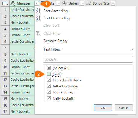
Step 9: Filter out the null rows in the Manager column as these are redundant Bonus Bands. Click on the drop-down beside the Manager column > deselect ‘null’ from the list:
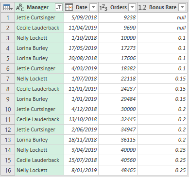
Now the table contains the Bonus Rates for each row:
For Bonus Points (no pun intended!)
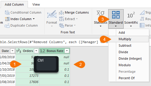
Step 10: If you want to go the extra mile you can add a calculated column for the Bonus amount. Select the Orders column then hold down the CTRL key and select the Bonus Rate column. On the Add Column tab > select Standard > Multiply:
Step 11: Rename the column; double click the header and type in a new name. I’ve called the column ‘Bonus’:
Power Query Approximate Match VLOOKUP Dates
This approach will also work with dates. For example, the blue table below lists fiscal quarters:
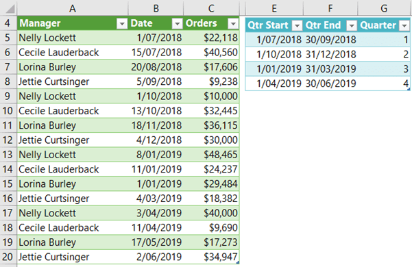
I can easily assign them to the Order table by merging them and following the same steps above. Download the workbook to see the complete example.

have two tables
One table has date and remark as below
Date Remark
31-Dec-21 2021 Orders
30-Jun-22 Jan – Jun 2022 Orders
31-Dec-22 Jul – Dec 2022 Orders
30-Jun-23 Jan – Jun 2023 Orders
31-Dec-23 Jul – Dec 2023 Orders
Second table is sales order table as below
Sales Order Order Date
620101820410 22/12/2021
620101820420 22/06/2022
620101820430 22/12/2022
620101820440 22/05/2023
620101820450 22/12/2023
If Order date is before 31-Dec-2021 then remark should be 2021 Orders which should be matched with first table.
I want to merge these two tables in power query with approximate match on order date with reference to remark table.
Please explain with syntax and table and example
Hi Hemal,
The data in table 1 needs to be split out into 3 columns: Start Date, End Date and Remark. Please post your question on our Excel forum where you can also upload a sample file and we can help you further.
Mynda
Power Query Approximate Match VLOOKUP with Dates very urgent, Please help.
Can you send me an example as you showed for order value and rate step by step.
Please post your question on our Excel forum where you can also upload a sample file and we can help you further.
If the source data changes, do you need to perform the fill again? or will it automatically update?
If the source data changes you just need to refresh the query and it will update the output.
It is also possible to use lists to evaluate the bonus rate. The steps could be as follows:
1) in two separate queries, transform each column of the BonusRates table into lists called OrderValue and BonusRate
2) in an empty query, create custom function fnBonusRate using Advanced editor:
(Orders as number) as number =>
let
Selection = List.Select(OrderValue, each _ <= Orders),
Position = List.Count(Selection) – 1
in
BonusRate{Position}
List.Select function creates another list called Selection containing only those OrderValue <= Orders. The number of items in the Selection list decreased by one is the position of the desired bonus rate in the BonusRate list.
3) add new column BonusRate, either as a Custom column =fnBonusRate([Orders]) or as Invoked custom function
For Orders <10000, the custom function results in error – it is possible to solve it by adding zero OrderValue band into BonusRates table or add a condition for the custom column =if [Orders] < OrderValue{0} then null else fnBonusRate([Orders]) or just ignore it.
The advantage of this solution is that it retains the original rows order in the table. For very large data sets it may be less efficient because it transforms each Orders value separately (I did not test it).
P.S.: Thank you for the great blog, I often use it as a source of inspiration.
Thanks for sharing, Vladimir.
Hi Mynda,
Alternative solution you might like, is simply appending both tables, sorting on the lookup column and filling down the result columns. I learned this trick from your colleague Oz.
BTW loved what you did for Excel Hash 2018 challenge.
Ooh, that’s clever too. Thanks for sharing!
Note for others, the lookup columns need to have the same column name so they are appended in a single column for the purpose of the sort.
I figured there had to be a way to do this in Power Query but I hadn’t yet looked into it – I use vlookup with the TRUE as the final argument with date ranges all the time, and I wanted a way to do that in Power Query. This is a great solution! Thank you!!!
Glad you found it helpful, Yvonne 🙂
perfect thank you
Glad it was helpful 🙂