Since VLOOKUP is one of the most popular Excel functions it makes sense that one of the first things you want to do in Power Query is VLOOKUP. But step away from the Add Custom Column button because there’s not a formula in sight.
Excel Power Query VLOOKUP is actually done by merging tables. Makes sense if you think about it, after all a VLOOKUP is simply pulling a column from one table into another table.
This tutorial applies to Excel 2010 onwards and requires the Power Query add-in, or if you have Excel 2016 you'll find it on the Data tab in the Get & Transform group.
The Data
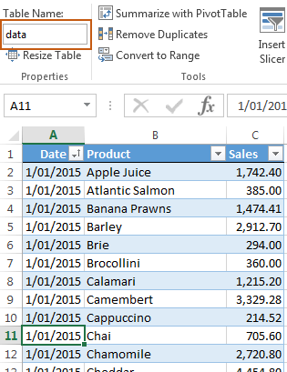
Our data is in a simple table called “data” (nothing like stating the obvious), containing a date, product name and sales amount:
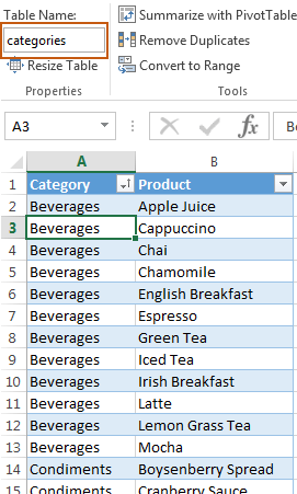
We have a lot of different products and I’d like to group them into categories so they’re easier to analyse.
In comes table number 2, called “categories”, which maps my products into their respective categories:
An aside, if you were to use VLOOKUP formulas to bring the Category name into the "data" table you’d have to either switch the column order in the "categories" table so Product was in column A and the Category in column B, or use INDEX & MATCH, or some other clever manipulation of VLOOKUP to make it lookup to the left.
Not with Power Query, it's not fussy about column order, as you'll see.
Excel Power Query VLOOKUP
- Format your two tables as an Excel Table (CTRL+T and make sure they have headers)
- Load the data table into Power Query: Excel 2010/2013 Power Query tab > From Table, or Excel 2016 Data tab: Get & Transform group > From Table
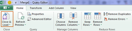
- Close the Query: Home tab > Close and load to > Connection only
- Repeat steps 1 through 3 for the categories table
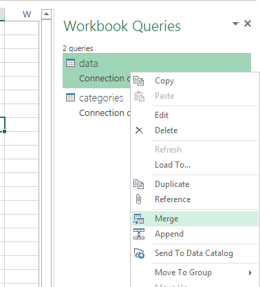
- In the Workbook Queries pane in Excel right-click the data query > Merge:
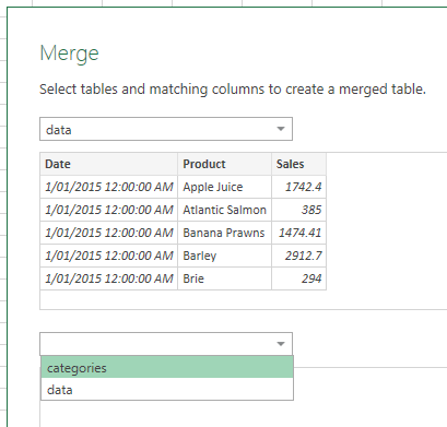
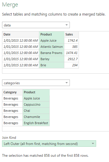
- In the Merge dialog box select the categories table in the bottom section:
- Left click your mouse on the Product column in the data table. It should turn green.
- Left click your mouse on the Product column in the categories table. It should also turn green. This tells Power Query which columns to match up.
- The Join Kind will default to ‘Left Outer’ which is fine since I want to make sure all of the records in my first table (data) are retained even if there isn’t a corresponding category for a product.
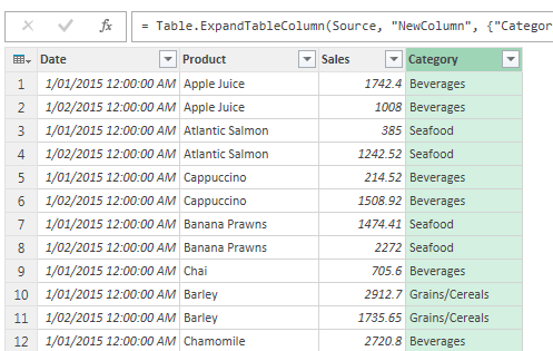
Click OK, which will open the Power Query editor window:
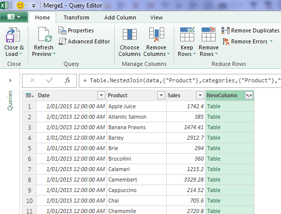
You can see we have the first table (data) in the first 3 columns and then a NewColumn which is effectively our second (categories) table.
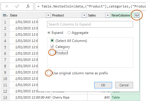
- Click on the double headed arrow on the NewColumn. This displays a list of columns in the categories table. Uncheck the Product column since we already have this in our data table. Also uncheck the ‘Use original column name as prefix’ and click OK.
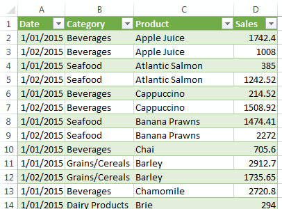
- Now we have a new table which includes the product category column:
- I’ll do some tidying up:
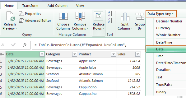
- Drag the Category column in between the Date and Product columns
- Format the Date column as Data Type: Date:
- Format the Sales column as Data Type: Currency
- Close and Load To a Table:
And now you have a new table in an Excel worksheet containing your 4 columns ready for analysing in a PivotTable or formulas.
I know that seems like a lot of steps but it actually only takes around 1 minute to set it up when you know what you're doing, as you can see in this video (no sound):

And the best thing is if your source data changes (new data, new categories, new anything), you can update the query by clicking the Refresh button on the data tab.
Download the Workbook
Enter your email address below to download the sample workbook.
Power Query VLOOKUP Approximate Match
Replicating a VLOOKUP Exact Match formula in Power Query is easy, as you've seen above, however replicating a VLOOKUP Approximate Match formula in Power Query isn't, but that's a post for another day.
More Power Query
The Definitive Guide to Power Query; what it's good for, what versions of Excel can get it, where to download it and more.

Very useful. Thanks.
Great to hear, Patrick!
all videos are so nice and simple to understand.
Great to hear, Jiky!
I have a shared workbook that is being used by multiple user on OneDrive. Users have been complaining that they find it difficult to update if someone else is using the file. I’ve put this file in Power Query and created a query for each them.
My challenge is how do I connect all the three queries to the original workbook(master file) so that each teams updates is captured in the master file? I would love to hear your inputs. I’m new to power query. Not sure what it can and cannot do yet. Thanks.
Hi Vhena, please see this tutorial on getting data from OneDrive or SharePoint with Power Query. If you get stuck please post your question on our Excel forum where you can also upload a sample file and we can help you further.
I have merge 3mil rows data, but a new merge query has only 500,000 rows.
Can you help me with this problem?
Hi Tuoi,
we can help.
Can you describe the problem and provide the code you are using?
Use our forum to create a new topic, will be easier to help you there.
Catalin
I was trying to use vlookup and then index match, none of those worked but did not know about power query and how it was lurking in the background all along, waiting for it to being used. Thank you for opening the gates to a whole new world in excel!
Great to know you discovered Power Query, Nick!
Thank you Mynda. I need to combine data from different workbooks and am currently using Vlookups to do this. Is it possible to do this using Power Query?
Sure is 🙂 Just create a query for each workbook, then merge them as required.
Is it possible to bring the category without creating another merge table query? If I bring to refer many tables to bring the information, in this case I will need to create merge query one by one for each table. Instead I would prefer to bring fields from various table into my first table without creating merge query table.
Hi Nishant,
You can merge the primary table with others. You don’t have to ‘Merge as new’, instead choose ‘Merge’.
Mynda
OMG. I love this! I’ve been trying to use index match on two criteria (userid and month) to extract the the team they were on for that month (individual productivity by team by month). Inner joining on name and month (CTRL while selecting columns) worked perfectly! You’re a life saver!
🙂 glad I could help, Matt!
=VLOOKUP(I1,$A$1:$E$4,3,FALSE)*J1 +VLOOKUP(K1,$A$1:$E$4,3,FALSE)*L1+VLOOKUP(M1,$A$1:$E$4,3,FALSE)*N1
Please let me know how use array formula
Hi,
After you type the formula in a cell, instead of pressing the Enter key to exit formula editing, press these 3 keys in the same time: Ctrl+Shift+Enter. This will also exit formula editing, but it will enter the formula as an array formula, by automatically wrapping the formula in curly brackets.
Hi Mynda,
In your example, let’s say you wanted to exclude Seafood and Beverages. Would it make sense to take care of that in the categories query? Or just pull all entries in, and then filter the Categories column within the merge? Since I had already done the former, my merge preview shows ‘null’ for corresponding entries, as they’ve been filtered out previously. This isn’t a problem, except now I’ll need a second filter in the merge to get rid of the nulls. Wondering from a best practice and performance perspective- redundant filtering, but fewer records brought in, or bring in all records and filter once? Thanks!
Hi Jeff,
I would merge then filter. Power Query doesn’t bring data into anywhere until you Close & Load. All you see in the query editor is a preview, so there’s no real efficiency gain to do the filter before or after.
Mynda
This is great! My only question is why is Power Query returning more rows than the Data table. For example, my Data table is huge (about 1,000,000 rows.) My “Categories” table has about 70,000 rows. Since the merge is simply adding another column into the Data table, why is the output table more than the 1,000,000 rows? The only reason I even noticed this is because I got a warning message that there were too many rows for Excel to handle. (over the 1,048,576 row limit.)
Hi Mary Ann,
The merge must be resulting in duplicate rows. This might be caused by multiple rows in table A matching multiple rows in table B.
Mynda
This is such a lifesaver as I’m a big fan of VLOOKUP and your opening statement matches what I felt when I try to use it in Power BI. Thank you for sharing this on your blog.
You’re welcome, Suhaila 🙂
Hi Mynda,
I’m anxiously awaiting your post about replicating a VLOOKUP Approximate Match formula in Power Query! Have I missed that one? Is it in the works?
I’ve been searching all over the web for it and found a few “solutions” but nothing as clear and concise as I’m sure your post will be. What I found were more like workarounds.
Any way you can help me out? Any links you can share?
Thanks!
Dave
Hi Dave,
No, you haven’t missed it. I’ll email you when it’s available. You could try this approach.
Mynda
Hi,
This explanation was amazing but I have a problem since I currently tried to merge two queries since using the lookup formula.When I select the first table (query) to merge into the other Query (both are in the same excel file) it have been taking me out around 141 rows, so for this reason when I compare my results are not the same.
How can I fix this issue. I am merging these two queries using the column PO – Invoice but it is not considered the entire data.
Could you please let me know?
Hi Leyman,
Make sure the same data type is set for that column in both queries.
I suggest opening a new thread on our forum, with a sample file attached, so we can evaluate the problem.
Great post Mynda with clear instructions, it saved me a big amount of time searching how the merge function was working !
Perfect Christmas gift 🙂
Thanks !!!
Marc
Glad I could help 🙂
Hi Mynda,
It is a great way to merge data you have explained in your video. However, when performing the merge I always get duplicated records. Would you be able to suggest have any solution to that?
Hi Peter,
I’d say something is going wrong in step 8 or 9 or both. Difficult to tell without seeing your file. Please post your question on our Excel forum where you can upload your file so we can help you further.
Mynda
Hi Mynda,
You are correct. Problem appears on step 9. I will raise a question on your forum.
Thank you,
Peter
I followed these instructions, but when I expanded the table in the merge query, the rows were randomly re-arranged. I fixed this by adding an Index column as the first step.
I just learned about Power Query yesterday, and this was amazingly helpful to me, thank you!
Glad I could help, Mary. Have fun with Power Query 🙂
I have Match replicating VLOOKUP Exact Match, but can’t figure out a way to have it replicate Approximate Match. Any thoughts?
Hi David,
use: “*” & LookupValue & “*”, the asterisc wildcard will allow for partial matches, can be any text before or after the lookup value. If you want to allow only prefixes or suffixes, remove the corresponding wildcard.
Catalin
Good tutorial Mynda.
As an aside, I worked through the example and it works well! No surprise! No but … !
For no real reason I left the two tables as two tables and added them to the data model. I then created a relationship between the two tables using Product in both cases. I know you know this but it works exactly the same as the merged table solution you are presenting here.
FYI
the merged tables solution is 161Kb on my W10 Excel 2016 system
the relationship solution is 227 Kb on the same system
Duncan
Hi Duncan,
Yep, that’ll work if you have one table with a column of unique values and if that table contains all instances of the product. Might not always be the case.
Power Pivot is good at compressing large amounts of data, less so with small tables like in this example.
Cheers,
Mynda
I liked this. Thank you. A power query for you: How can I do this same thing but base the “lookup” off the first few characters. For example, I would like to merge but on all values that START WITH “AMZ”. Is this possible? Thanks.
Hi Alex,
Power Query merging doesn’t allow for partial matches. You’d need to split the AMZ etc. into a different column so you can match the entire column.
Mynda
Hi. I’m new to Power Query but I can see that it would make my job so much easier. I am facing a dilemma though, mainly on making sure that each column has the right data within it. Isn’t Power Query supposed to recognize a column based on a column name, not on its order in the worksheet? For example, I’ve got a file with names, ages and gender (in that order with columns named accordingly) and another file with names, grades, ages and nationalities (also in that order with columns named accordingly). When I append or merge the files or load from a folder, the table shows the data from the two files in the same order that the columns are arranged. Consequently, column 2 will have a mixture of ages and grades, and so on.
How can this be avoided without having to go into each file to fix the column order?
Thanks.
Power Query doesn’t match column names when you append or get data using ‘From Folder’. It’s up to you to ensure your data structure is identical for these techniques.
Alternatively, you can get each file in a separate query and then merge the queries. When you merge you can specify which columns match so you don’t end up with a jumble of data.
Mynda
Thanks for this Mynda.
I’ve been looking at using PowerQuery and PowerPivot for processing my bank and credit card statements, rather than my existing formula-based approach. I’m very impressed with these tools and want to work with them more – if I can work out how to use them in my real-life scenarios. They just seem a powerful and sophisticated approach, and I prefer using built-in tools than extensive personal customisation – and I view extensive macros and formulae as effectively customisation that comes with the ‘cost’ of having to continually update them as things change.
One of the major issues for me arises with categorisation. Consider the ‘Categories’ table in the example. Every single item (product) has to have a row here that matches the product name exactly, whereas a formula-based or macro-based approach can check for substrings (e.g. a company name) within the item string (product name) and assign the appropriate category.
Do you have any ideas how categories can be assigned on a similar basis in a PowerQuery/Pivot approach?
Thanks in advance
Hi Stephen,
Great to hear you’re interested in Power Query and Power Pivot. They are amazing tools.
Power Pivot won’t allow you to create relationships between tables unless there is an exact match, so to speak.
Power Query has functions which can find substrings. e.g. Text.Contains Text.StatsWith Text.EndsWith so you may be able to utilise them in your model. You’d have to write some custom functions to look through a list of ‘categories’ to see if they are within the text string, so it’d be some pretty advanced M code.
Mynda
Thanks for the tips Mynda.
These powerful tools seem to have been rather quietly slipped into Excel as far as most Office users are concerned, and I’m only just beginning to explore them – which is why I’m following your posts.
I am honestly amazed how much database-like functionality Microsoft has been able to introduce into Excel. MS Access showed us what a mess the average user makes of a true database product, but tools like Power Pivot make such powerful functionality usable by average Excel users.
I was unaware of these Power Query functions, so I’ll take a good look. Perhaps I had better spend some time reading a few tutorials to get a balanced understanding of Power Query and Power Pivot capabilities, rather than trying to pick them up by trial and error.
As to the macros, hopefully I will be to start from those I wrote to do multiple searches from such “a list of ‘categories'” when the number of searches meant that a single formula was getting ridiculously long.
Thanks again, and keep up the good work
Yes, Excel has come a long way now that we have the Power tools.
I don’t advise trying to pick them up by trial and error. Power Pivot in particular needs to be set up the right way from the outset, or you’ll find yourself rebuilding it from scratch if you get it wrong.
I can recommend some courses ;-p
https://www.myonlinetraininghub.com/excel-power-query-course
https://www.myonlinetraininghub.com/power-pivot-course
Mynda
Hi Mynda,
Is there any chance you could add a link to download the source data file so we can follow your instructions and check we get the same answer?
Thanks
Hi Mark,
You can download the workbook here.
Mynda
This is awesome information. Thank you so much for sharing this. I know I’ll be using this one in the future.
Thanks, Glenda. Glad you’ll find it useful.
Mynda
Step 12 tidying up, you state:
“Format the Date column as Data Type: Date:”
But in the green table below the numbers in that column still don’t have $ or € or …. signs in front of them.
Hi Paranam,
The ‘formatting’ in Power Query is different to that in Excel. In Power Query it is setting a data type. This helps Excel know whether the data is text, numbers etc., but more importantly it helps Power Pivot know what type of data it is as well.
I cover this in more detail in my Power Query and Power Pivot courses.
In Excel the formatting you have available is a cosmetic appearance on the cell, it doesn’t affect the underlying value contained within that cell. It also offers you the ability to use other characters in the format, like currency symbols etc.
Kind regards,
Mynda