TEXTSPLIT, TEXTBEFORE and TEXTAFTER Functions

It’s been a long wait, but we finally have some exciting new Excel text functions that are going to make life so much easier. In this tutorial I’m going to focus on TEXTAFTER, TEXTBEFORE and most exciting, TEXTSPLIT. The first two functions are fairly self-explanatory, and so is TEXTSPLIT to a degree. However, in this tutorial I’m going to show you some cool tricks that aren’t immediately obvious and aren’t covered in Microsoft’s documentation.

Note: At the time of writing these functions are currently only available to Microsoft 365 users on the Insider channel, but hopefully they’ll be generally available to all Microsoft 365 users soon.

UPDATE: since filming this tutorial these functions have had additional arguments added to them as a result of feedback received while in the beta testing phase. The written tutorial below has been updated, but the video is based on the original function syntax. All examples, except example 5 for TEXTSPLIT, still apply with the updated syntax.

Watch the New Excel Text Functions Video

Download Workbook

TEXTAFTER Function

The TEXTAFTER function extracts the text from a string that occurs after the specified delimiter.

Syntax: =TEXTAFTER(text, delimiter, [instance_num], [match_mode], [match_end], [if_not_found])

input_text	The text you are searching within. Wildcard characters not allowed. Required.
delimiter	The text that marks the point after which you want to extract. Required.
instance_num	The nth instance of text_after that you want to extract.  By default, n=1.  A negative number starts searching input_text from the end. Optional.
match_mode	Determines whether the text search is case-sensitive. The default is case-sensitive. Optional. Enter 0 for case sensitive or 1 for case insensitive. Optional.
match_end	Treats the end of text as a delimiter. By default, the text is an exact match. Optional. Enter 0 to not match the delimiter against the end of the text, or 1 to match the delimiter against the end of the text. Optional.
if_not_found	DValue returned if no match is found. By default, #N/A is returned. Optional.

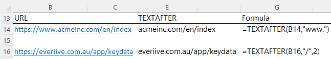
For example, we can extract the domain name onwards from the URLs below. Note the formulas are different depending on whether they have www. In front of the domain name:

TEXTBEFORE Function

The TEXTBEFORE function extracts the text from a string that occurs before the specified delimiter.

Syntax: =TEXTBEFORE(text, delimiter, [instance_num], [match_mode], [match_end], [if_not_found])

input_text	The text you are searching within. Wildcard characters not allowed. Required.
delimiter	The text that marks the point before which you want to extract. Required.
instance_num	The nth instance of text_after that you want to extract.  By default, n=1.  A negative number starts searching input_text from the end. Optional.
match_mode	Determines whether the text search is case-sensitive. The default is case-sensitive. Optional. Enter 0 for case sensitive or 1 for case insensitive. Optional.
match_end	Treats the end of text as a delimiter. By default, the text is an exact match. Optional. Enter 0 to not match the delimiter against the end of the text, or 1 to match the delimiter against the end of the text. Optional.
if_not_found	DValue returned if no match is found. By default, #N/A is returned. Optional.

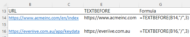
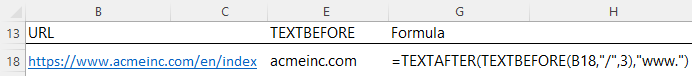
And if you want to extract just the domain name you can wrap TEXTBEFORE in TEXTAFTER:

TEXTSPLIT Function

The TEXTSPLIT function splits text strings using column and, or row delimiters.

Syntax: =TEXTSPLIT(text, col_delimiter, [row_delimiter], [ignore_empty], [match_mode], [pad_with])

input_text	The text you want to split. Required.
col_delimiter	One or more characters that specify where to spill the text across columns. Optional.
row_delimiter	One or more characters that specify where to spill the text down rows. Optional.
ignore_empty	Specify TRUE to create an empty cell when two delimiters are consecutive. Defaults to FALSE, which means don't create an empty cell. Optional.
match_mode	Searches the text for a delimiter match. By default, a case-sensitive match is done.
pad_with	Text entered in place of blank results.

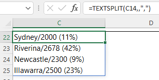
We’ll use the text string below in the TEXTSPLIT function examples. You can see it has several delimiters we can use including forward slash, space, comma and parentheses.

Sydney/2000 (11%),Riverina/2678 (42%),Newcastle/2300 (9%),Illawarra/2500 (23%)

Note: The above text string is in cell C14 and will be referenced in the examples below.

Example 1.1 - Split text by comma delimiter across columns:

An easy way to split this string is by comma delimiter and we can write that formula like so:

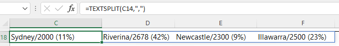
Notice it spills the results to columns C:F in a dynamic array. We can then reference this array using the array spill operator # as follows: =C18#

Example 1.2 - Split text by comma delimiter down rows:

Notice the two commas after C14 instruct Excel to skip the col_delimiter argument.

Example 2.1 - Split text by comma delimiter and forward slash across columns:

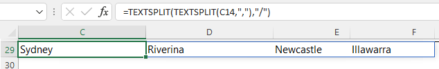
Notice the data after the forward slash is discarded.

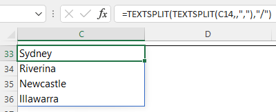
Example 2.2 - Split text by comma delimiter and forward slash down rows:

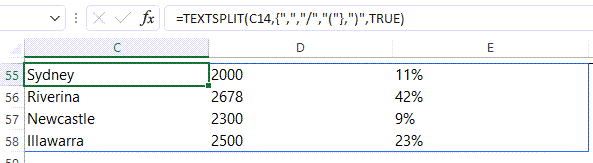
Example 3 - Split text by all delimiters down rows:

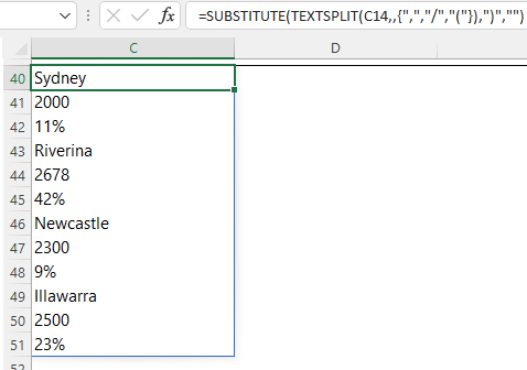
In this formula the TEXTSPLIT function does the bulk of the work:

=SUBSTITUTE(TEXTSPLIT(C14,,{",","/","("}),")","")

Notice the delimiters have been entered in an array constant with curly braces:

=SUBSTITUTE(TEXTSPLIT(C14,,{",","/","("}),")","")

And then the SUBSTITUTE function cleans up the closing parenthesis:

=SUBSTITUTE(TEXTSPLIT(C14,,{",","/","("}),")","")

Example 4 - Split text into rows and columns:

Here I’ve used both the row and column delimiters. This formula also requires TRUE in the ignore_empty argument to ensure the spacing of the results is correct.

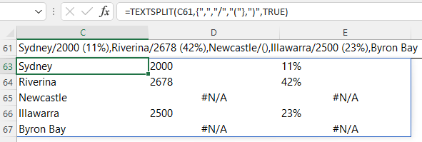
Example 5 - Handing errors:

In this example we’re using a slightly different text string shown in cell C61 in the image below. Notice Newcastle is missing data and ‘Byron Bay’ on the end also has no data and none of the delimiters, which results in errors:

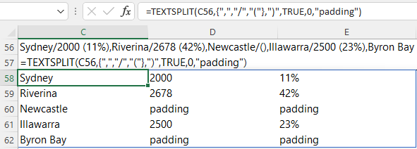
The last argument in the TEXTSPLIT function is ‘padding’ and we can use this field to hide or replace errors returned by gaps in the data with something else. In the example below I’ve entered the word ‘padding’ so you can see.

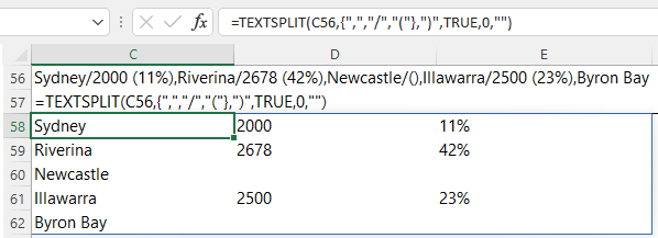
Alternatively, you can enter two double quotes to simply hide the errors: