Excel Factor Entry 3 Re-format Data Using Formulas

July 4, 2012 by Mynda Treacy

Importing data into Excel from other systems rarely goes without the need to fix formatting before you can even use it.

Sandy R from Pittsburgh, PA sent in this Excel Factor entry.

Using the REPT, LEN, FIND and MID functions Sandy can transform thousands of rows of data that comes into Excel like this:

3707.314278
17001.0048655
51898.315006

To a xxxxxxx.xxxxxxx format like this:

0003707.0314278
0017001.0048655
0051898.0315006

Let’s say Sandy’s data is in column A and formatted as Text (this is important for the formula to work). The formula she uses looks like this:

=REPT(0,7-LEN(MID(A2,1,FIND(".",A2)-1)))&MID(A2,1,FIND(".",A2)-1)&"."&REPT("0",7-LEN(MID(A2,FIND(".",A2)+1,LEN(A2))))&MID(A2,FIND(".",A2)+1,LEN(A2))

Yikes! Actually it’s not that scary. Let me translate it into English;

Find the characters in front of the full stop, count how many characters there are, then take the number of characters up to 7 by adding zeros to the front of the characters in front of the full stop. Then add a full stop. Do the same for the characters after the full stop.

Obviously Excel doesn’t solve the formula in this order but I think it helps to know that this is what you are trying to achieve.

To understand how it works we’ll take a look at each function in the first part of the formula (up to the &MID...) using the first item in Sandy's list (3707.314278) as our example:

FIND Function

The FIND function returns the starting position of one text string within another text string. FIND is case-sensitive.

=FIND(find_text, within_text, [start_num])

In Sandy’s formula she is finding the location of the full stop like this:

FIND(".",A2)

The result: 5 i.e. the full stop is the 5^th character.

Note how Sandy hasn’t entered a start_num argument. This is because the start_num is optional. You can tell it is optional because it is in [square brackets].

The start_num is the character you want to start the search from. The first character in within_text is 1. If the argument is omitted it will start at the beginning of within_text.

MID Function

The MID function returns the characters from the middle of a text string, given a starting position and length.

=MID(text, start_num, num_chars)

In Sandy’s formula:

=MID(A2,1,FIND(".",A2)-1)

The result =MID(A2,1,5-1)

The end result are the first 4 characters: 3707 (these are text not numbers)

LEN Function

The LEN function returns the number of characters in a text string.

=LEN(text)

Sandy’s uses MID and FIND to tell Excel which text she wants to find the length of.

=LEN(MID(A2,1,FIND(".",A2)-1))

The result: =LEN("3707."-1)

=LEN(5-1) i.e. how long is the text up to and including the full stop, then take 1 off so that we don't count the full stop.

REPT Function

The REPT function repeats text a given number of times.

=REPT(text, number_times)

In Sandy’s formula:

=REPT(0,7-LEN(MID(A2,1,FIND(".",A2)-1)))

This section of the formula evaluates to:

=REPT(0,7-LEN(5-1))

=REPT(0,3) i.e. repeat the zero 3 times.

Sandy then uses the ampersand (&) with MID to concatenate her new text together with a full stop in between.

&MID(A2,1,FIND(".",A2)-1)&"."&

The second half of the formula is slightly more complicated because it needs to start after the full stop, but now that you know how MID, FIND, LEN and REPT work you can figure out the rest for homework 🙂

The Non-Formula Approach

Now, if you want a less brain intensive option that’s only slightly more laborious you could do it this way:

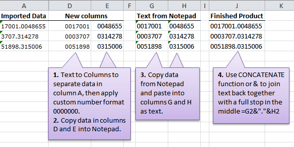
Use Text to Columns to separate the two halves of the data using the full stop as a delimiter.
Apply a custom number format 0000000 to your two new columns D and E.
Copy the new data and paste it into Notepad (free in your Windows Accessories folder).
Copy it out of Notepad and paste it back into Excel as Text (Paste Special > Text).
Use CONCATENATE or the ampersand to join the text back together with a full stop in between. Ok, so it uses one tiny formula.

Excel Tidy up Data

Note: if this is something you have to do regularly then it is worth taking the time to get your head around a formula like Sandy’s as this is the quickest long term solution.

Thanks for sharing your mammoth formula with us, Sandy.

Sandy R works for a law firm in Pittsburgh, PA and does a combination of IT and Library Science duties. She has used Excel for the last eight years, not only in her current job but also in previous jobs.

Vote for Sandy R

If you’d like to vote for Sandy’s tip (in X-factor voting style) use the buttons below to Like this on Facebook, Tweet about it on Twitter, +1 it on Google, Share it on LinkedIn, or leave a comment….or all of the above 🙂

AUTHOR Mynda Treacy Co-Founder / Owner at My Online Training Hub

CIMA qualified Accountant with over 25 years experience in roles such as Global IT Financial Controller for investment banking firms Barclays Capital and NatWest Markets.

Mynda has been awarded Microsoft MVP status every year since 2014 for her expertise and contributions to educating people about Microsoft Excel.

Mynda teaches several courses here at MOTH including Excel Expert, Excel Dashboards, Power BI, Power Query and Power Pivot.

Excel Factor Entry 2 – AutoFilter

Excel Factor Entry 4 INDEX and MATCH Two Criteria

Comments

Pooja

April 25, 2013 at 6:47 am

I have a text that looks looks this:
R1_LUT X,Y 0.3, -1.7 OR at time can also look like this:
R1_LUT X,Y -0.3, -1.7
I want to extract 0.3 as well as -0.3, using one robust formula, because the numbers could appear with signs OR without signs.
I used the mid function =MID(A64,14,4) and it works well, but for the string in the first line, I end up with 0.3, and I don’t need the comma here.
Can someone help me with using a conditional MID function, that will take care of both scenarios, to give me 0.3 as well as -0.3
- Mynda Treacy
  
  April 25, 2013 at 8:12 pm
  
  Hi Pooja,
  
  If you want to extract the 0.3 and -0.3 as text you can use this formula:
  
  =IF(ISNUMBER(FIND(“-0.3”,A2)),-0.3,MID(A2,12,3))
  
  If you need them to be numbers then you can wrap the above formula in the VALUE function like this:
  
  =VALUE(IF(ISNUMBER(FIND(“-0.3”,A2)),-0.3,MID(A2,12,3)))
  
  Where A2 contains your text.
  
  Kind regards,
  
  Mynda.
  - Pooja
    
    April 26, 2013 at 1:54 am
    
    Hello Mynda.
    Wow! Thanks for your reply.
    However, my numbers could be anything, not just a 0.3 or a-0.3.
    i.e. I am looking to make this more generalized:
    R1_LUT X,Y 0.3, -1.7 So—R1_LUT X,Y is always going to appear in the line, but the two set of numbers could be anthing as well as could be signed or unsigned(but will always be seperated by commas)
    Can you help me with a more generalized formula, using comma as a leverage in the formula?
    - Mynda Treacy
      
      April 26, 2013 at 10:11 am
      
      Hi Pooja,
      
      If I were you I’d use the Text to Columns tool as opposed to writing a long complex formula that has to handle multiple scenarios. If the last letter before your value is ‘Y’ you can use ‘Y’ as the delimeter which will give you the last half of your text, then you can run it through text to columns again and use the comma as the delimeter to get rid of the text on the end.
      
      Let me know if you get stuck.
      
      Kind regards,
      
      Mynda.
      - Ram Porwal
        
        May 17, 2013 at 8:06 pm
        
        Hi Pooja,
        
        You can use below formula.
        
        =VALUE(TRIM(RIGHT(LEFT(A1,FIND(“,”,A1,FIND(“Y”,A1))-1),4)))
        
        hope it will help you.
        
        regards,
        Ram Porwal
Steve

March 1, 2013 at 6:36 am

Since this manipulates the data as text only, it might have been better if you used text in the example, and not number that were going to be treated as text by Excel. Just to avoid confusion.

With that said, how do I accomplish the same feats that I would use ‘mid’ for, but having the output be usable numbers, and not numbers that Excel thinks is text? (I ended up having to do a “a1+a1-a1” game to convince Excel that what was in the a1 cell was actually a usable number.)

Any insight?
- Carlo Estopia
  
  March 1, 2013 at 3:55 pm
  Hi Steve,
  
  What do you mean exactly by “a1+a1+a1”? As far as I know, and as what I’ve double-checked– your
  complaint–, I don’t get that type of result unless through concatenation “a1&a1&a1”. But
  adding texts would result VALUE# error.
  
  Anyway, even as texts, numbers get treated as numbers by excel except that they’re indented
  to the left instead of to the right.
  
  But I’m not closing this one without a neat solution:
  Data E5: 12432
  Use INT or VALUE(if you have decimals)
```
=INT(MID(E5,1,3)) or  =VALUE(MID(E5,1,3))
=INT(MID(E5,1,4)) or  =VALUE(MID(E5,1,4))
result: 4 + 3
All indented to the right and behaving like numbers
as they should.
```
  OR….
  
  Maybe, you need to:
  1) Go to Excel Options
  2) Click Advanced
  3) Scroll down to : Display options for this worksheet
  4) Uncheck: Show Formulas in cells instead of their
  calculated results
  5) It would also help by copying and pasting them as values
  and converting them to numbers/numeric formats.
  
  Cheers.
  
  CarloE
Karine Bouffard

October 31, 2012 at 12:17 am

Nice tip indeed! I tried to re-use some of it for a problem I have at work but did not manage to make it work! I need to only select part of the text written as below:
US60/TAT520,423
US60/PEL588N,508
I would like to extract only the middle text TAT520 or PEL588N. The issue is that the number of letters or figures are not always the same. Only “US60/” and “,423” is fixed (text or figures can change but it’s always 4 letters or figures + / and ,+3 figures). I managed to extract only TAT520,423 using =MID(D5,FIND(“/”,D5)+1,LEN(D5)-4) but I could not get rid off the ,423 too. Would you know how to do this Mynda?
Thanks for your help.
Karine
- Mynda Treacy
  
  October 31, 2012 at 7:12 am
  
  Hi Karine,
  
  In your case I would use the dead-easy Text to Columns. I say in your case because you have two consistent delimiters; the forward slash and comma.
  
  More on Text to Columns here.
  
  Kind regards,
  
  Mynda.
- Mike
  
  January 29, 2013 at 10:37 pm
  
  We could use the combination of MID, FIND and CHAR.
  
  The ASCII Value for:
  “/” is Char(47)
  “,” is Char(44)
  
  Let say your data are in cells:
  A1 US60/TAT520,423
  A2 US60/PEL588N,508
  
  Try this formula in cell B1:
  =MID(A1,FIND(CHAR(47),A1)+1,(FIND(CHAR(44),A1)-1)-FIND(CHAR(47),A1))
  
  I know it is very late (haha), but I hope it could help others in the future.
  - Mynda Treacy
    
    January 30, 2013 at 10:22 am
    
    Cheers, Mike. Thanks for sharing. 🙂
Raju

July 4, 2012 at 1:22 pm

It is a very good tip. I liked the second one (Non-Formula Approach) because my end users are not that much formula savy.

Thanks for sharing such a nice tip. Keep posting.

Raju Padaria
FAG Bearings India Ltd.
Vadodara (India)
P & I Schaeffler, India
Business Excellence
- Mynda Treacy
  
  July 4, 2012 at 1:30 pm
  
  Thanks, Raju 🙂

Excel Factor Entry 3 Re-format Data Using Formulas

FIND Function

MID Function

LEN Function

REPT Function

The Non-Formula Approach

Vote for Sandy R

More Excel_Factor Posts

More Text Formulas Posts

More Excel Formulas Posts

Reader Interactions

Comments