The need to look up and match multiple criteria is quite common; however as with most things in Excel there are many ways to ‘skin a cat’, I'll share two options with you here.
Matt Duncan from Florida sent in this a cool INDEX and MATCH array formula that allows you to match two criteria from two separate columns and return the corresponding value.
Thanks for sharing, Matt. I don’t recall ever seeing the MATCH function used this way.
Beware, you may need a Brain-booster (a healthy fruit or vegetable snack they get my 6 year-old’s class to eat at about 9.30am to help them concentrate), or a strong coffee, whichever you prefer.
I’ll show you Matt’s impressive formula, and then I’ll show you how I cheat with a non-array approach using VLOOKUP.
Enter your email address below to download the sample workbook.
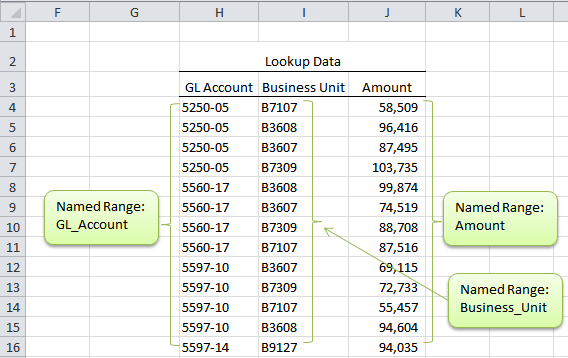
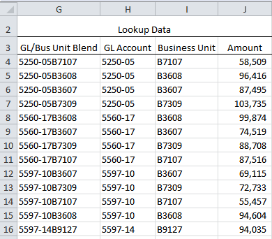
Here’s the data Matt is looking up (Note: this is a simplified version for the purpose of this tutorial):
The above table has the following Named Ranges because it’s quicker to build the formula and easier to follow:
Range H4:H16 = GL_Account
Range I04:I16 = Business_Unit
Range J4:J16 = Amount
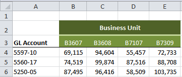
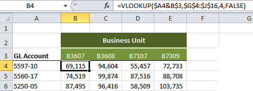
Here’s the table Matt wants to populate (also simplified):
So, you can see that Matt needs to match both the GL Account and Business Unit which are in separate columns in the Lookup Data table, and then return the corresponding amount from column J in the lookup data.
Here is Matt’s formula from cell B4 (we’ll refer to cell B4 for the remainder of this tutorial):
=IFERROR(INDEX(Amount,MATCH(1,($A4=GL_Account)*(B$3=Business_Unit),0)),0)
Note: this is an array formula so you need to enter it with CTRL+SHIFT+ENTER to get the curly brackets at each end that you see below. This is what you see in the formula bar when you enter it correctly:
In English it reads:
Return the Amount from column J that corresponds with GL Account 5597-10 in column H, and Business Unit B3607 in column I, if you don’t find it return a zero.
Let’s take a closer look at the MATCH part of Matt’s formula because that’s where the magic is happening.
How the MATCH Function Part Works
First, remember the MATCH function searches for a specified item in a range of cells, and then returns the relative position of that item in the range.
The twist is that Matt has two specific items he wants to match, the GL Account and Business Unit.
The syntax for the MATCH function is:
=MATCH(lookup_value, lookup_array, [match_type])
Lookup_value – the value you want to find
Lookup_array – the column/row containing the value you want to find
Match_type – optional argument represented by a -1, 0 or 1.
- -1 finds the smallest value that is greater than or equal to lookup_value,
- 0 finds the first value that is exactly equal to lookup_value, or
- 1 finds the largest value that is less than or equal to lookup_value.
Here’s the MATCH component of Matt’s formula:
=MATCH(1,($A4=GL_Account)*(B$3=Business_Unit),0)
Note how he has two lookup_arrays:
1. GL Account column ($A4=GL_Account)
2. Business Unit (B$3=Business_Unit)
And how, instead of using the lookup_value as his criteria to match, he has entered the criteria in with the lookup_array.
I have never seen that before!
So, How Does It All Work?
Array formulas are testing for TRUE or FALSE outcomes and award them a numerical equivalent of 1 for TRUE, and 0 for FALSE.
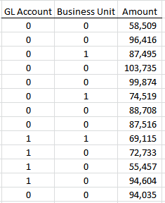
The MATCH part of the formula evaluates each cell in the GL_account column and if it matches the GL Account code in A4 (5597-10) is awards it a 1, and if it doesn’t it awards it a zero.
It does the same for the Business_Unit column, matching B3607 to give you an array like this:
Or in a formula it looks like this:
=MATCH(1,{0,0,0,0,0,0,0,0,1,1,1,1,0}*{0,0,1,0,0,1,0,0,1,0,0,0,0},0)
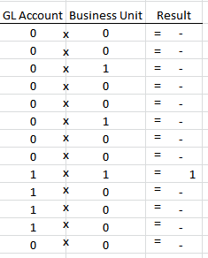
Which is the same as doing this calculation:
Since the only row resulting in a 1 is on row 9 of the array, the MATCH component of the formula evaluates to 9, which is used by the INDEX function as the row number argument.
So, let's take a look at the INDEX function part of the formula now.
INDEX Function
Remember the INDEX function in the array form returns the value of an element in a table or an array, selected by the row and column number indexes.
And the syntax for the INDEX function in the array form is:
=INDEX(array, row_num, [column_num])
Array – the range of cells containing the data you want to find.
Row_num – the row number your data is on.
Column_num –the column number your data is in.
Matt’s formula evaluates to this:
=INDEX(Amount,9)
The column_num argument is optional, and since there is only one column in the Amount Named Range the argument is not required.
For icing on the top Matt then wraps his formula in an IFERROR function so if a match is not found a zero will be entered in the cell instead of an error.
Here is Matt's formula one last time
=IFERROR(INDEX(Amount,MATCH(1,($A4=GL_Account)*(B$3=Business_Unit),0)),0)
The VLOOKUP Cheat
Now, if the carrot I gave you didn't help and all that array business still did your head in, I’ve got a simpler option that requires a helper column.
Some would say the helper column is cheating 😉 but I say go with the path of least resistance, unless of course it is worthwhile in the long term, which it is for Matt.
Remember the reason Matt couldn’t use a regular INDEX & MATCH formula or VLOOKUP is because both of these can only look up/match one value.
So, an alternative solution is to create a unique value in your lookup data from the two columns you’re trying to match i.e. the GL Account and Business Unit, by joining them together. This is where the helper column comes in.
In the table below I have a new column (G) that CONCATENATES (joins) the GL Account and Business Unit values together using a formula in cell G4 like this:
=H4&I4
The result is what you see below in column G.
Now you have your unique GL/Business Unit identifier you can use a VLOOKUP formula like this:
=VLOOKUP($A4&B$3,$G$4:$J$16,4,FALSE)
Which evaluates like this:
=VLOOKUP(5597-10B3607,$G$4:$J$316,4,FALSE)
For more on using VLOOKUP to find multiple criteria.
To eliminate potential errors wrap it in an IFERROR function like this:
=IFERROR(VLOOKUP($A4&B$3,$G$4:$J$316,4,FALSE),0)
Note: whilst array formulas are effective they can also be taxing on your system memory. If you have a lot of data to search through the VLOOKUP option may be more efficient.
Thanks for sharing your cool trick and teaching me something new, Matt.
Matt Duncan is an accountant for a global payroll processing company located in Florida. He has no formal training in Excel but loves to find new ways to use Excel’s vast functionality.
“As you can imagine, a payroll company has limited time to complete all the processes that go into producing a single pay check not to mention a batch of 30,000 checks!
There are numerous ways to make a mistake on a pay check and with only a few hours to produce a check and fund the hundreds of benefits, vendors, governments and garnishments, etc., there is a constant need for process improvement.
One of the most time consuming processes has been funding verification. With global corporations clients sharing a payroll cycle between all its companies the verification process included manual inputs based on a variety of filtering and VLOOKUP’s. The process could take up to 2 hours depending on the number of accounts and the number of companies included in a pay cycle just to input data!
My role is to audit all the pay cycles at the end of the month and report back to the client with any errors and, of course, improve processes that can cause errors, i.e. manual inputs!”
Vote for Matt
If you’d like to vote for Matt's tip (in X-factor voting style) use the buttons below to Like this on Facebook, Tweet about it on Twitter, +1 it on Google, Share it on LinkedIn, or leave a comment….or all of the above 🙂



Interesting way of doing it. If the data has more than 1 match, will it retrieve only the first number?
What if you used sumifs() ?
Hi Don,
If your objective was to summarise values then yes, SUMIFS would be the tool for that, however if you wanted to lookup text values then SUMIFS wouldn’t work.
Mynda
Hi,
I am trying to write an INDEX formula with four conditions, i am trying to pull DEPRECIATION amount for a specific Cost Centre, for a specific account for a specific month. I am working with about 9000 lines there are no duplicates. example (Amount, Cost Centre number, GL account and the corresponding month. I have tried to write it but i am getting either #N/A or #VALUES obviously I am doing something wrong.
Hi Precious,
Please use our Help Desk to upload a sample of your calculations, this way we can see where the problem is without guessing.
Don’t forget to give all the details, even create a sample of desired result. I will gladly help you to solve this problem.
Thanks for understanding 🙂
Catalin
I cannot for the life of me get an index match formula with 2 criteria to work.
I am using named ranges and either get N/A or Value errors. Commas in the Match produce Value, equal signs produce N/A.
=INDEX(rngCovers,MATCH(1,(A2=rngSaleDate)*(B2=rngSaleLocation),0))
What is wrong with this formula? Any help would be appreciated.
Hi Paula,
Have you entered it as an array formula with CTRL+SHIFT+ENTER?
Kind regards,
Mynda.
Mynda, Thanks A LOT ! Finally, I succeed in creating a right formula, thanks to your explanations and Matt formula 🙂
You’re welcome, Parda 🙂 Glad we could help.
This could be done by using SUMIFS
=SUMIFS(Amount,Business_Unit,B$3,GL_Account,$A4) Using the same named ranges.
Cheers, Jude. You are correct. However if the data you wanted to find was text instead of values, SUMIFS wouldn’t work, whereas Matt’s solution and the VLOOKUP cheat would.
Kind regards,
Mynda.
=IFERROR(SUMPRODUCT(($A4=GL_Account)*(B$8=Business_Unit)*(Amount)),0)
copy the above across and down, and this should do the same function. I would send the spreadsheet but not sure how!
Hi Ibrahim,
Send it here: HELP DESK
Cheers,
CarloE
Thank you very much Matt.
Thanks a lot Mynda.
You’re welcome, Ahsan 🙂
please ignore my previous comment or request and concider the following. sorry for any inconvienience that this might cause.
Please help regarding the following issue.
I am working for the capital market regulator of maldives. I am dealing with statistics maintained by regulator regarding the Maldives Stock Market. I have got to calculate the maximum fee the brokers, stock exchange and regulator have earned on share transaction for this year.
We have three level of fees approved by the regulator. The following are the three level, (MVR means Maldivian Ruffiyaa)
1. If the transaction value is > or = to MVR 50,000.00 the brokers may charge maximum 1.5% of the transaction value as Brokerage commission + maximum 0.5% of the transaction value as trade processing fee for the stock exchange.
2. If the transaction value is > MVR 50,001.00 and or = MVR 100,001.00 the brokers may charge maximum 0.5% of the transaction value as Brokerage commission + maximum 0.5% of the transaction value as trade processing fee for the stock exchange.
basically I want to develop a formula which includes all the above three conditions applicable to the transaction value. For an example I have a 3 three columnar table where the first column or Column A has X number of Transaction Value(s) where each cell has one transaction value, second Column or Column B should have the brokerage commission(s) charged for each corresponding transaction value in Column A considering all the three conditions mentioned above and third Column or Column C should have the trade processing fee(s) charged for each corresponding transaction value in Column A consider three conditions mentioned above.
Hi Muslih,
I see that your logic is incomplete,
for example how much will be charge for beyond 100001 MVR?
Anyways, here’s your formula
Here’s your logic:
IF Transaction value is <=50000
Brokerage commission 1.5%
Processing fees .5%
Elseif Transaction value is >= 50001 and <= 100001
Brokerage commission .5%
Processing fees .5%
Question: What if beyond 100001? Hence, your formula
will return a false value.
NESTED IF
Cheers,
CarloE
correction of second level.
2. If the transaction value is > MVR 50,001.00 and or or = to MVR 100,001.00 the brokers may charge maximum 0.5% of the transaction value as Brokerage commission + maximum 0.5% of the transaction value as trade processing fee for the stock exchange.
Dear Mynda,
Thank for sharing, hope you wont mind I asking, what if I have both 2 account in column-H, can you advice me on how can I get the total $$ of 5250-05B7107 5251-05? ( $18+$50+$45)
column-G , column-H, column-J
5250-05B7107 5250-05 $10
5250-05B7608 5250-05 $30
5250-05B7107 5251-05 $18
5250-05B7107 5251-05 $50
5250-05B7608 5250-05 $30
5250-05B7107 5251-05 $45
5250-05B7107 5250-05 $18
Best regards,
William
Hi William,
You need the SUMIFS function.
IF you only have Excel 2003 then you can use an array formula or SUMPRODUCT.
Array entered with CTRL+SHIFT+ENTER:
SUMPRODUCT:
Kind regards,
Mynda.
You are my master, Much appreciation.
Big THANK YOU
^_^
Hi,
I just have a similar question. in a excel file I have 2 colums (Column C: authors name, and column D: is the corresponding published articles).
each author may have different articles for instance Carl may have 5 articles and Johana has 15 articles and so on.
I want to make a list that under name of each authors we have a list of his/her articles summarized.
I have used the below formula for retriveing the first Match
and the formula below for second Match
But it is not working for third and other articles corresponding to each author.
In this file I have 2 columns (author name and corresponding projects) comprising a few rows (for simplicity.)I want to make a table that reads from these two columns ( which in reality may exceed 200 rows) and check when the authors name in cell for example I4 (Carl) matches the author name in the range of column C then write the corresponding projects.
if you apply these fromulas you can see in this example Carl has 4 work that I can auto detect them by the first two formulas but not more than these two. Can you please see if you can help me to match the rest of papers for each article.
I need a formula that checks the same procedure perhaps but ignores these 2 previous detected and written works but detects the new corresponding work.
Many thanks in advance.
an excel file is availabe to be sent if need be.
Best Regards,
Ashkan
Hi Ashkan,
A better tool would be a PivotTable. If you want to send me your file I’ll insert a PivotTable for you as an example.
Kind regards,
Mynda.
Hi,
I have more simpler non-array formula which I learned from one of my colleagues in Daniel’s ‘Excel Hero Academy’ class which does the same job =INDEX($J$4:$J$16,MATCH(H4&I4,INDEX($H$4:$H$16&$I$4:$I$16,),0))
Above formula can be altered with named ranges as in the sample workbook =INDEX(Amount,MATCH(H4&I4,INDEX(GL_Account&Business_Unit,),0))
Cheers, Syed 🙂
Thanks for posting all of the tips, and the training you provide. It sure is a lot of help to newcomers like me. I was just asking some one how to do this yesterday. Keep up the good work. And way to go Matt and Mynda!
Thanks, Jeanette. Glad we could help.
Kind regards,
Mynda.
Holy cow this is deep- thanks for the coffee warning and the post. So great to know there are other self taught individuals out there- Thanks, Matt and Mynda!
You’re welcome, Chris 🙂
Perhaps I’m missing something… but if he used Excel 2007 and up, couldn’t he just use the SUMIFS function to populate that table? No need to activate array formulas…
=SUMIFS([sum range],[category range1],[value1],[category range2],[value2])
Hi Miroslav,
Yes, you are correct. You can also use SUMIFS in this example. Note: if the data you wanted to find was text instead of values, SUMIFS wouldn’t work, whereas Matt’s solution and the VLOOKUP cheat would.
Thanks for sharing. Pat on the back to you too 🙂
Kind regards,
Mynda.
Hi, Theoretically, great formula. Has lot of things to learn. However, could this not be easily obtained by using the Pivoting – as shown here under:-
Sum of Amount Column Labels
Row Labels B3607 B3608 B7107 B7309 B9127 Grand Total
5250-05 87495 96416 58509 103735 346155
5560-17 74519 99874 87516 88708 350617
5597-10 69115 94604 55457 72733 291909
5597-14 94035 94035
Grand Total 231129 290894 201482 265176 94035 1082716
Thanks & Regards,
Raghu
Hi Raghu,
Yes, correct. You could do the same with a PivotTable. In Matt’s case he needed to populate another more complex table that wasn’t as simple as my example, and so the formula suited him better.
Thanks for sharing. Pat on the back to you 🙂
Kind regards,
Mynda.
Thank you for the cool tricks. It really helps.
You’re welcome, KM007 🙂