This Excel Factor tutorial was sent in by Bryon Smedley of Bristol, Tennessee.
Suppose you receive a spreadsheet with calculations, but the calculations are stored as text, for display purposes only, and not used to actually derive answers.
Without wanting to reinvent the wheel, you decide to try and use the documented versions of the formulas as actual number crunching tools.
Let’s set the stage for how this is accomplished.
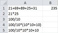
The spreadsheet looks something along these lines:
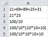
Since there are no equal signs in front of any of the equations, Excel interprets them as simple text strings.
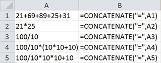
If you would like to know the answers to these equations, but retain the original text in Column A, a common approach would be to use the CONCATENATE function to produce the following functions in Column B:
 |
OR |
 |
Unfortunately, this does not work and yields the following result.
Because the original data was seen as text, the CONCATENATE function does not attempt to perform any sort of calculation and merely connects the two text strings together.
This is where an old, forgotten Excel 4.0 function comes into use: the EVALUATE Function.
EVALUATE is an Excel v4.0 macro function which is still packaged and supported in Excel 2010. The EVALUATE function allows for the evaluation of a text equation as an algebraic equation.
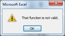
The odd thing about the EVALUATE function is that it cannot be used directly in a cell, like SUM or AVERAGE. The function can only be utilized with the confines of a NAMED RANGE. If you attempted to use it in the following manner, =EVALUATE(A1), you will be presented the below error message.
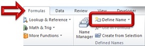
The trick is to program the EVALUATE function as a NAMED RANGE and then call the name from the target cell. This is how the process works:
- Select cell B1
- Go to the FORMULAS tab and click Define Name
- In the New Name dialog box, type the name Result (this can be any valid range name you like)
- In the Refers to: box type: =EVALUATE($A1)
- Click Add then OK.
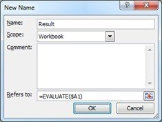
It is very important to note that you select cell B1 and used a Relative Row reference for $A1.
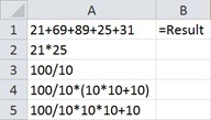
Now enter =Result into cell B1 and copy it down for the remaining cells.
 |
 |
 |
|
(1) First Pass |
(2) First Answer |
(3) Fill Down |
Keep in mind, since this is actually an embedded Excel macro, you must save the file as an Excel Macro-Enabled Workbook (.XLSM) file.
USING THIS IN EVERYDAY SITUATIONS
Now that we understand this new (albeit old) power, how can it be used in more typical scenarios?
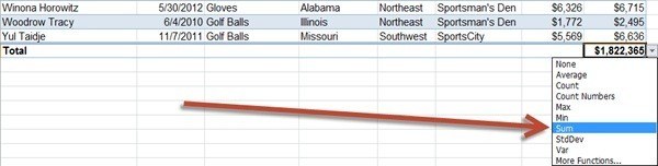
Excel 2007 introduced us to an improved version of Tables which have this wonderful ability to create formulas on the Totals line with convenient drop-down lists.
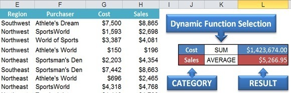
That’s great and easy, but what if we want that same drop-down functionality in a traditional table, or we want to have the drop-down located at the top of the data (or anywhere for that matter?)
Excel 2007/2010 Data Tables function selection drop-down
Data Table functionality at top of sheet
|
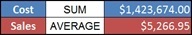
We want to be able to go from one set of formula choices… |
|
|
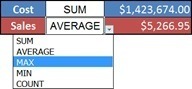
…access a drop-down list of alternate choices… |
|
|
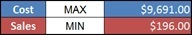
…and dynamically create a new summary of calculations. |
|
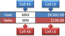
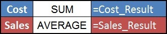
The steps are the same as outlined above, but in this case we need to distinguish between the Cost (column "G" data) calculation and the Sales (column "H" data) calculation.
To simplify matters, we will add the entire column so the user can add data to the table and the calculations will still work.
|
Place your cursor in cell L5 and create the following Named Range |
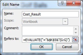 |
|
Place your cursor in cell L6 and create the following Named Range |
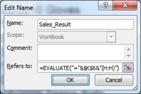 |
IMPORTANT: Because we will not be filling this functionality down cells, and each cell points to a different data range, the reference pointers must be completely absolute. $-signs in front of the column letter and the row number.
The final step is to type =Cost_Result in cell L5 and =Sales_Result in cell L6
Enter your email address below to download the sample workbook.
Thanks again, Bryon for putting in so much effort to write this tutorial and include loads of images to help us follow along. We appreciate you sharing your knowledge.
Bryon is from Bristol, Tennessee and has been teaching Excel since version 7 which was included with Office 95. He is currently a Technical Training Analyst for one of the largest coal companies in the world. His key responsibility is to conduct all Microsoft Office training, but in addition he also serves as a technical consultant for any and all projects involving Microsoft Office applications.
Bryon says “Excel is by far my favorite among all the Office applications due to the almost infinite number of situations it can be used. There literally seems to be no end to its usefulness.
My favorite Excel tools are difficult to narrow down. Without getting into third party add-ins, I would have to say PivotTables (especially with the addition of Slicers. WOW! Are those things awesome!!), the Text to Columns tool (what a time saver), and Macros.”
Vote for Bryon
If you’d like to vote for Bryon’s tip (in X-factor voting style) use the buttons below to Like this on Facebook, Tweet about it on Twitter, +1 it on Google, Share it on LinkedIn, or leave a comment to thank Bryon for taking the time to share his knowledge….or all of the above 🙂

I defined a name Like This:
=EVALUATE ( OFFSET ( INDIRECT( “RC”,FALSE), 0 , -1 ) )
It evaluates from the left cell wherever you use it.
Thanks for sharing, Samuel!
I have Office 365 and Evaluate doesn’t seem to work the way you describe anymore. I can only specify what I want to evaluate in the Name Manager. Naming a specific reference while calling the defined name in a cell doesn’t work. Example: if I define a name Result with Refers to: Evaluate($A1) and then type in cell B1 =Result(A1) I get an error #VALUE!. However if I just call =Result it will properly evaluate the formula in A1 however I am thus unable to evaluate a formula in any other cell with this same named function.
Hi Andrew,
I think you’re a little confused. It doesn’t say to use =Result(A1), it says =Result
You also need to ensure you select cell B1 before you define the name because this is a relative named range i.e. it’s relative to the cell in which you use it. More on relative named ranges here.
I hope that clarifies things, but shout if you have more questions.
Mynda
Doesn’t seem to work well with workbook reference. My original formula works without opening source file, but once I use Evaluate method it shows #Ref error until I open source.
(There are other reasons why I can’t use original formula)
EVALUATE can’t reference a closed workbook. Perhaps you can post your question and sample Excel file on our forum where we can help you find an alternate solution.
Mynda
Hi,
This tool is great, and is very close to solving my problem – it its automatically updating ie when the target workbook cell is updated and both documents saved the =Evaluate named range does not update. I have to double click the cell with the =evaluate named range to get it to update. Any ideas how to fix this?
Hi Sean,
Try to add a volatile function to the Evaluate function, like =YourFormula+Now()*0
The NOW function is volatile, will be recalculated at each excel recalculation.
Cheers,
Catalin
Thank you for sharing 🙂
Thank you very much for the well explained topic as well as the details in others questions below.
I tested this solution and it works like a charm for what I intend to do while I am using simple funtions, however, when I try to put on some matrix referencing formulas, or even quite a few conditionals, it starts to give me #value errors.
Other thing that would be really really awesome is if I was able to use this kind of funtion on other areas such as in imput formula for conditional dropdown lists in cells, or conditional formatting.
Would anybody know if there are limitations of arguments to use the Evaluate funtion, and if there is any way to implement it in lists or conditional formatting?
Thanks !!
Yes, there is a limit of 255 chars per string evaluated, if your formula text exceeds this limit, the Evaluate function will fail.
You can use it anywhere you like, but I’ve never seen this function in a conditional formatting formula, you can build very complex formulas without the need of Evaluate. However, you know best what scenario you have, if you feel it’s easier with Evaluate, then use it, the final result is what matters.
Catalin
Thank You for taking the time to post this most helpful tip. I hope that you have a blessed day.
Does this work on Excel for Office 365 on a Mac? I have version 15.32 and it looks like they have done away with the ability to have the referenced range ($A1 in the case above) be a formula.
I also wasn’t able to find the evaluate formula on my version of Excel.
Any thoughts would be appreciated.
Thanks!
Hi,
As described in this article, Evaluate is not a sheet function, it’s an Excel 4 macro function, that can be used in a defined name, not in a cell directly.
I am not aware if Microsoft still supports old macro functions for Mac 2016, but you can test that very easy: Type in cell A1 the value 1, in cell A2 type 2, then define a new name(TestEvaluate), with this formula in the Refers To field: =Evaluate(“=A1+A2”). In any cell, type this formula: =TestEvaluate . If this cell displays the correct result, you have support for excel 4 macro functions.
Mac 2016 does not support Evaluate function. Terribly unfortunate.
I am using it in a Virtual Desktop now, and the Evaluate function is supported, and I was able to get the correct answer per your TestEvaluation idea above.
However, I am now trying to evaluate a named range that refers to =EVALUATE (Sheet1!L17) when the contents of cell L17 is (text) “= ‘\\apkvf01\ tsredirect$\ kohlman\ Desktop\ [Test 2.xlsx] Sheet1’!A4”.
I am trying to pull data out of a closed document, and I cannot open the document. It is part of a bigger project.
Thanks!
Hi Kohlman,
I’m pretty sure the EVALUATE function doesn’t work with closed workbooks. I say ‘pretty sure’ because there is very little documentation on this function since it’s not officially supported.
Mynda
Hey Kohlman,
Seems that what you’re trying to do can be accomplished by using power query. I was struggling with having to get data from several workbooks without needing to open them. Well, power query does just that!
Hi Didson,
Indeed, Power Query can do that and more, now. This post was written in 2012, before Power Query was around 🙂
Mynda
I’m trying to use this method with a formula that contains a file path to an outside workbook. I can get your example to work using as you outlined but when I try the following I get a value error:
AVERAGE( IF (‘R:\CRC\ AA-DL-UA Stopsale\ DL Stopsale\ [02-02-17 DL Stopsale.xlsx] Stopsale’!$C:$C = C2, IF ( ‘R:\CRC\AA-DL-UA Stopsale\ DL Stopsale\ [02-02-17 DL Stopsale.xlsx] Stopsale’!$D:$D = D2, ‘R:\CRC\ AA-DL-UA Stopsale\ DL Stopsale\ [02-02-17 DL Stopsale.xlsx] Stopsale’!$Q:$Q,””) ) )
Hi Dan,
Have you tried with the other workbook open? From your formula, seems that the workbook is closed.
Catalin
I used this to method to create a formula string to reference a cell in another spreadsheet.
=CONCATENATE( “=VLOOKUP(Q1,'[DriverLoans-“, A4, “.xlsx]Sheet1′!$A$1:$D$100, 3, FALSE)” )
Where A4 is the name of the driver. It works fine as long as I go to a cell, enter the defined name that EVALUATES the above formula, then hit Enter. But I expected it to AUTO REFRESH each time the DriverLoans-[driver].xlsx is updated, without having double click or F2 (edit) the cell then Enter. At the least, I expected it to REFRESH each time I open the spreadsheet or manually refresh.
I even created a Macro to record a series of F2, then Enter, to mimic a manual update, but the Macro resulted in putting blank in the cells. Which is bizarre because manually doing it works. But recording the manual steps in a Macro causes it to put blank in the cells.
I already saved it as a .xlsm and turned all all automatic updates in the FILE OPTIONS menu.
Is there a way to make this automatically update or is there another way that allows for automatic update?
Hi Ronnel,
You can try adding a volatile function like Now(), these type of functions are recalculated each time. Adding NOW()*0 to your formula will not change the result of your calculations. If your formula is expected to return text strings, not numbers, then adjust it to your needs, to add a zero length string instead of a zero: IF(Now()*0=0,””,0)
Catalin
Hi Mynda
Very helpful trick for Dashboard. I am facing one issue, I have a name range for few cells and I wants to use this EVALUATE, however I am not able to get correct result. For Example, Range Name is MyRange for cell A1:A10 value of which is 1, 2, 3,…, 10 I wants to calculate SUM, MAX, MIN, AVERAGE, COUNT – selection from Data Validation List
I created Name Range EVAL with following formula:
=EVALUATE (“=”& Sheet2!$B$2&” ( “&MyRange)
I selected SUM from List, I wrote in “C2” as =EVAL and I got SUM result as 2 instead of 55 and if I write =EVAL in “C3” then I am getting SUM value as 3 instead of 55
I modified EVAL as follows
=EVALUATE (“=” & Sheet2!$B$2& ” ( “&MyRange&” ) “)
But same result
Will you please help?
Thanks
Chirag
Hi Chirag,
Can you please upload a sample file on Help Desk? It will be very helpful to see what you did there and to understand where the problem is.
Thanks for understanding.
Catalin
Hi Chirag,
The Evaluate function will not accept a named range, you have to provide the reference as a text: A1:A10.
If you provide a named range instead of a text reference, Excel will create your function for the A1:A10 range (which contains numbers from 1 to 10) like this:
{“=SUM(1)” ; “=SUM(2)” ; “=SUM(3)” ; “=SUM(4)” ; “=SUM(5)” ; “=SUM(6)” ; “=SUM(7)” ; “=SUM(8)” ; “=SUM(9)” ; “=SUM(10)”}
There is a way to convert back the name to a text reference, but it involves another excel 4 macro function:
Use this in your EVAL name:
=EVALUATE(“=”&Sheet1!$B$2&” ( “&REFTEXT(MyRange,Sheet1!$A$1) &” ) “)
The REFTEXT function will convert your named range to a text, and the Evaluate function will be able to calculate the entire range, not only the implicit intersection:
This is what Evaluate function will receive from REFTEXT function:
{“=”&SUM&” ( “&”A1:A10″&”)”}
This way, you will be able to use a dynamic range inside Evaluate function.
Cheers,
Catalin
Love this function, wish it were a regular function that allowed nesting.
However, Evaluate function does not seem to auto-calculate. Does anybody have a solution for this?
Joe
Hi Joe,
Use a simple trick: use a volatile function to force a recalculation every time excel recalculates, without changing the result of your calculations: =EVALUATE($A1) +NOW()*0
NOW()*0 will always be zero, so it will not affect your result, but this function is volatile, so it will be recalculated every time a cell changes.
Cheers,
Catalin
Thank you very much. But I have this problem: If it is written A2+A3 in cell A1 (in your example) and I change value in source cell (A2 or A3 in your example), the value in B2 is not re-evaluated automaticly. I must press Ctrl+Alt+F9. I would like to make set of formula choices. But I dont want to press Ctrl+Alt+F9 after every change in source cells. Can you help me, please?
Thank you once more.
Martin
Hi Martin,
Is the calculation mode set to Automatic? Check this setting, can be found on Formulas tab, Calculation section, select Automatic from Calculation Options.
Let us know if this was the problem.
Cheers,
Catalin
Hi Catalin, thanks for your answer. The calculation mode is set to Automatic. All of formulas are calculated automatically, only formulas with Evaluate function aren’t.
Best regards
Martin
Hi Martin,
A volatile function must be recalculated whenever calculation occurs in any cells on the worksheet. A nonvolatile function is recalculated only when the input variables change. EVALUATE is a nonvolatile function, it will be recalculated only when you make changes to the text in A1, as it’s not directly dependant to A2 or A3!
In VBA, it’s easy, we can add Application.Volatile to make an UDF volatile:
Function EVALUATEString(ref As String)Application.Volatile
EVALUATEString = EVALUATE(ref)
End Function
You can try this version of VBA EVALUATE function. Use it in sheet cells like this: =EVALUATEString(A1)
But there is a way to make a nonvolatile function volatile: for this, we have to use a VOLATILE function (like NOW() function )in our defined name:
=EVALUATE(Sheet6!$A1) + NOW()*0
Of course, i had to multiply NOW with 0, to keep the original calculation intact.
Hope it’s clear 🙂
Regards,
Catalin
It´s super trick! (…+NOW()*0).
Using VBA Function EVALUATEString helped me too.
Thank you very much, my problem is solved and I learned new knowledge of Excel.
Martin
You’re welcome Martin 🙂
Thank you so much for this, you really saved us!
You’re welcome, Cary. Glad we could help.
Thank you. It was excellent and helped me much.
You’re welcome, S 🙂
NICE THANKS,BUT SAME NAME IS NOT WORKING IN OTHER SHEET (MULTIPLE) WITH IN SAME WORKBOOK
Hi MMI,
I’m not sure what you mean. If you’d like to send me your workbook via the help desk I can take a look at the problem.
Kind regards,
Mynda.
HI MYNDA
THANKS, FOR YOUR PROMPT RESPONSE.I WILL SEND YOU MY FILE.
Could have never guessed! Has been of great help in my work. Thank you.
When you create formulas with text functions, and you added to the formula the equal sign, for example =25+34, like in the fourth figure that is in the post. Also works if you use command find and substitute de equal sign for another equal sign, then Excel will transform the text formula into a formula.
Hi Ricardo,
Nice Info right there.
Thank you.
CarloE
Thanks, Bryon and Mynda!
For VBA developers only – you can read an interesting fact about Evaluate function and UDFs here:
Formula to change another cell
Cheers,
Kris
Thanks, very informative to know about old formula quirks.
Often though I resolve this problem by doing the following:
1. Select the column that has the concatenated values such as =21*25
2. Do a Copy paste special values of selection
3. Data text-to-columns and finish
Thanks,
Gordon
Cheers, Gordon.
I agree, Text to Columns is a great tool and the one I would probably use to fix the formatting too.
Kind regards,
Mynda.
But doesn’t that remove the entire dynamic nature from the spreadsheet? Wouldn’t you need to re-Copy/Paste and re-Text to Columns every time the formulas changed?
If it was a single pass through the data, I can see your point, but my purpose was to provide a means of changing the questions (re: formulas) with no further work on the user’s part.
Have a great day!
Correct. I was considering a one-off change to fix the data but, if the intention is to add more data then your solution would be better. Good point.
Cheers.
Thanks for sharing, I have been learning a lot about excel. God bless you
Sincerely
Lupe Jau
Computer Instructor
Thanks, Lupe. Glad you’re enjoying learning from our site 🙂
Worth reading, thanks for sharing! 🙂