I received an email from Bill this week asking how he can check if a range of cells contains text or numbers, as opposed to being empty.
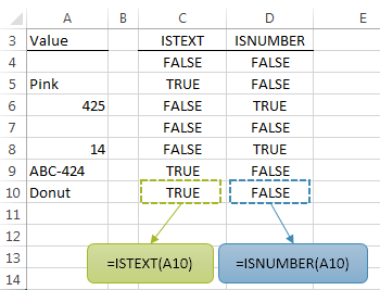
We can use the ISTEXT function to test for text, and ISNUMBER function to test for numbers, but these only work on one cell at a time.
Here’s the syntax:
=ISTEXT(value)
=ISNUMBER(value)
Where ‘value’ is the reference of the cell you want to test.
We can see them in action in the image below:
But Bill wants to test the whole range, A4:A10, to see if any cells contain text or numbers.
To check a range we can combine the ISTEXT and ISNUMBER functions with SUMPRODUCT like this:
=SUMPRODUCT(ISTEXT(A4:A10)+ISNUMBER(A4:A10))>0
In English it reads:
SUM the number of cells in the range A4:A10 that contain text + the number of cells that contain number values and if it is > 0 return TRUE, otherwise return FALSE.
So, how does this Beauty work?
Although this isn’t strictly an array formula, in that you don’t have to enter it with CTRL+SHIFT+ENTER, the SUMPRODUCT function behaves just like an array formula.
Let’s look at how it evaluates:
Step 1 – ISTEXT returns an array of TRUE/FALSE for each cell in the range A4:A10 like so:
=SUMPRODUCT((FALSE;TRUE;FALSE;FALSE;FALSE;TRUE;TRUE)+ISNUMBER(A4:A10))>0
Step 2 – ISNUMBER also returns an array of TRUE/FALSE for each cell in the range A4:A10 like so:
=SUMPRODUCT((FALSE;TRUE;FALSE;FALSE;FALSE;TRUE;TRUE)+(FALSE,FALSE,TRUE,FALSE,TRUE,FALSE,FALSE))>0
Step 3 – Now, since TRUE/FALSE have equivalent number values of 1 for TRUE, and 0 for FALSE when we apply the + to the two arrays inside the SUMPRODUCT function it converts them to their numeric equivalent like so:
=SUMPRODUCT((0,1,0,0,0,1,1)+(0,0,1,0,1,0,0))>0
Step 4 – SUMPRODUCT then adds the 1’s and 0’s together:
=SUMPRODUCT(7)>0
Step 5 – it tests whether the result of the SUMPRODUCT formula is greater than 0. If it is it returns TRUE, if not FALSE.
Array Formula Option
Of course we could achieve the same result from this array formula:
=SUM(ISTEXT(A4:A10)+ISNUMBER(A4:A10))>0
Although this is slightly shorter to write, remember because it’s an array formula we need to enter it with CTRL+SHIFT+ENTER.
Return a Different Message
If you want to return a ‘Yes’ or ‘No’, as opposed to the TRUE/FALSE outcomes, we can do this with an IF function like so:
=IF(SUMPRODUCT(ISTEXT(A4:A10)+ISNUMBER(A4:A10))>0,"Yes","No")
Test for Numbers Only
=SUMPRODUCT(ISNUMBER(A4:A10)*1)>0
Note the difference in this formula is the *1 after the ISNUMBER test. This is to coerce the TRUE/FALSE values into their numeric equivalents of 1 and zero.
We didn’t have to do this in the original formula because the + in the SUMPRODUCT function did that for us:
=SUMPRODUCT(ISTEXT(A4:A10)+ISNUMBER(A4:A10))>0
Another way to coerce TRUE/FALSE values is with the double unary like so:
=SUMPRODUCT(--ISNUMBER(A4:A10))>0
Test for Text Only
=SUMPRODUCT(ISTEXT(A4:A10)*1)>0
Or with the double unary:
=SUMPRODUCT(--ISTEXT(A4:A10))>0
Test if a Range is Empty
We can use the ISBLANK function to test if a cell is empty, but like ISTEXT and ISNUMBER, it only works on one cell at a time. The solution is to use SUMPRODUCT to test a range of cells and then compare the result to the number of cells in the range like so:
=SUMPRODUCT(--ISBLANK(A4:A10))=ROWS(A4:A10)
The ISBLANK function returns a TRUE for every blank cell, which we then coerce into the numeric equivalent using the double unary - -.
The ROWS function returns the number of cells (or rows) in a range.
In English it reads: SUM the number of BLANK cells in the range A4:A10, if it equals the number of ROWS in the range A4:A10 return TRUE, otherwise return FALSE
Using the original data as our example:
The ISBLANK formula evaluates like this:
=SUMPRODUCT({1,0,0,1,0,0,0})=7

=2=7

=FALSE
If the range A4:A10 were empty it would evaluate like this:
=SUMPRODUCT({1,1,1,1,1,1,1})=7

=7=7

=TRUE
Now, if you’ve read this far and are keeping up with me then you might be thinking, ‘can I use ISBLANK to test if any cells contain text or numbers instead of the original ISTEXT/ISNUMBER formula?’
The answer is yes, like this:
=SUMPRODUCT(--ISBLANK(A4:A10))<>ROWS(A4:A10)
In English: if the number of BLANK cells in the range A4:A10 is not equal to the number of rows in the range A4:A10 you will get TRUE, meaning there is at least one cell in the range that isn’t blank.
The downside of this option is the double negatives can do your head in, whereas interpreting the ISTEXT and ISNUMBER formula is a bit less draining on your brain power 🙂
Want to Learn Array Formulas?
Enter your email address below to download the sample workbook.
And if you really want to master them consider my Advanced Excel Course where I cover array formulas in detail, among other advanced Excel techniques.
Thanks
Thank you to Bill for inspiring this tutorial.

Thank you so much, solved my problem.
Cheers,
Dave.
Question:
Is there a way to then have the formula give the data in the cell that is not blank in that array? Ideally, it would give the intersection value between that cell and a cell in column B.
I have a set of data recording the results of a test. The participant receives a stimuli of a certain level and gives an answer. The cell for that level is then filled in with a y= yes or n = no. I want to translate these responses into a string of levels administered.
Hi,
Can you please upload a sample file on our forum, with some manual examples of the expected result? It will be much easier to understand your situation and provide quality help.
Catalin
Plz help on this below, need formula as we want is “2”
A418IN082486
A418IN082486
A418IN082486
A418IN082486
A418IN082487
A418IN082487
A418IN082487
A418IN082487
A418IN082487
A418IN082487
A418IN082487
in excel need formula
Hi Kumar,
What exactly do you want to do? It’s not clear.
Phil
ISTEXT(A1) shows TRUE but the Number Format is GENERAL and cell is empty
What could be the reason
Hi AZ,
Formatting to General has no impact on whether a cell contains text or now. That said, ISTEXT should only return TRUE if the cell contains a text string. I’d have to see the file to troubleshoot the cause in your case. If you want to upload your file and question on our Excel forum we’ll take a look.
Mynda
Works great. thank You.
Thank you!!! Finally found the correct formula to tell me if a range of cells had a value!
You’re welcome 🙂
This was spot on for my project today… thank you and God bless
You’re welcome.
Regards
Phil
I love your examples and guidance it really helps.
I have a unique question that is becoming complicated.
I have a spread sheet where one cell has multiple different words and I need to count the number of times each word is used, to come up with a number for each.
Course #
# Started With
# Finished With
# Graduated With
Released / Resigned/ Transferred 1 released 1 resigned 2 transferred
New Training Officer
# Transferred
Week Changed
Any suggestions:
Hi Dave,
Can you please upload a sample workbook with your data structure, and more details on what words you want to count?
Use our Help Desk to upload the file.
Cheers,
Catalin
Hi Mynda,
Your explanation helps me to understand how to look for a first numeric cell in a row.
However, after finding the first numeric cell, I need to continue looking for a second and a third numeric cell in a row. Is it possible to do this in a table where the first numeric cell is different from row to row?
Thank you!
Hi Rosa,
You can download this sample workbook for an example on finding the numeric cells: My Online Training Hub – Shared Files
The formula:
is an array formula, confirmed with CSE.
The formula is in cell J2, can be copied down and to right as needed. The COLUMN()-9 is meant to return the number of item from array of columns to be returned, to SMALL function. To return the first numeric cell column number, the second argument of SMALL function, -k-, must be 1. For column J, COLUMN() will return 10; COLUMN()-9 is 1 for column J, 2 for column K, and so on. This is a way of creating a dynamic parameter.
If you need to adjust the formula to your sheet, make sure to change the correction value to return 1 for the first numeric cell:COLUMN()-9 : for example, if you want to start from column E, this column number is 5, so this argument must be COLUMN()-4 to get the first cell…
Hope it’s clear 🙂
Catalin
Hi Mynda!! U r rocking…..its just beautiful….nice preparation with explanation…. No one can present more than this! awesome. U know this question is asked in interview written test paper recently which i attended.
Aw, thanks Emmanuel 🙂 Thanks for your kind words. I’m glad you like my tutorials.
S…Mynda! finally i found a very good techie cum teacher to clarify my doubts. Pls help me to know more about “Report Generation – Using Macros in Excel”. kindly send me some samples or show me your blog or lessons which you teached earlier.
Hi Emmanuel,
You can read all the past Excel tutorials on the blog.
Kind regards,
Mynda.
Hi Mynda,
This is a great explanation of how to use the sumproduct function and how it calculates. It is nice that you explained all the various possibilities of writing the formula to find the same result.
In regards to Ranjeet’s question, the double hyphen is actually a double negative. You can think of it as multiplying the values by negative 1 twice, resulting in a positive value.
-1 *-1 * value = positive numeric value
It is really just a shortcut to multiplying by one. I guess that pressing the hyphen key twice is faster than pressing asterisk and one keys.
The answers will be the same either way, but it is good to understand this when you work with someone else’s model.
Thanks again Mynda for presenting all the alternatives!
Hi Jon,
Thanks for your kind words…and for elaborating on the double unary/hyphen for Ranjeet 🙂
Cheers,
Mynda.
why we use double hyphen “–” in formula
Hi Ranjeet,
The double hyphen, or double unary as it’s called, coerces the TRUE/FALSE values into their numeric equivalents of 1 and 0. Without this coercion the function cannot apply the mathematical equation to the values.
e.g. if it’s the SUM function we need 1’s and 0’s in the array, not TRUE/FALSE. SUM cannot add TRUE/FALSE as these are not numbers.
Another way to coerce TRUE/FALSE values into their numeric equivalents is to multiply them by 1.
I hope that helps.
Kind regards,
Mynda.
This is why I enjoy reading your posts, even when it’s something I would have been able to figure out on my own. I would have thought about it more literally, and wouldn’t have come up with the sumproduct answer.
Here’s what I would have done (all are array-entered formulas):
Check if any cells contain text or numbers: =OR(ISTEXT(A4:A10),ISNUMBER(A4:A10))
Test for numbers only: =OR(ISNUMBER(A4:A10))
Test for text only: =OR(ISTEXT(A4:A10))
Test if range is empty: =AND(ISBLANK(A4:A10)) or =NOT(OR(ISTEXT(A4:A10),ISNUMBER(A4,A10)) or the simplest, =AND(A4:A10=””) (bonus — this one works with formulas that return an empty string; the rest will only work for truly blank formulas).
I think my way reads more logically to a layman, but your way is faster, plus it is safer if said laymen decides to mess around with the sheet…. I used Excel for over 10 years before I learned about the Ctrl+Shift+Enter combo!
Love it! Thanks for sharing, Bryan 🙂
I am having trouble and hoping you can help. I am trying to determine if any cell in a single row range has text and if so state yes otherwise no. For example:
Cells A2-E2 (range) and D2 has text, the output would be yes otherwise no. Likewise for multiples like text in A2, C2, and E2 would also output yes.
No matter what formula I try, it is not outputting correctly.
Hi Kristen,
You can use COUNTA to count instances of text/numbers in a row. If the count is > 0 then the row is not empty. e.g.
Mynda
Nicely Done! My head is still spinning, but I was able to follow it all.
Loved your “English Explanations” — very helpful.
Cheers, Tom 🙂 Sorry about the head spinning!