Excel Functions that Return References

Using a formula to return a reference to a range of cells allows us to generate a reference on the fly based on the shape of the data or criteria we specify. As our data grows these formula generated references can automatically update to include new data. This has huge efficiency advantages over hard coding the reference because we no longer need to edit formulas to update references when they change.

Many of us know the OFFSET function returns a reference to a range of cells, but there are actually 8 Excel functions that return a reference to a range:

1. OFFSET
2. INDEX
3. XLOOKUP (Excel for Microsoft 365 only)
4. CHOOSE
5. SWITCH (new in Excel 2019)
6. IF
7. IFS (new in Excel 2019)
8. INDIRECT

Each function has their pros and cons. Let’s take a look at them in turn.

Note: I’m not going to cover each function in detail. If you’re not familiar with any of the functions, there are links below to detailed tutorials.

Watch the Video

Download Workbook

Examples of Excel Functions that Return References

1. OFFSET Function

Step by step tutorial on the OFFSET function.

Syntax reminder:

=OFFSET(reference, [rows], [cols], [height], [width])

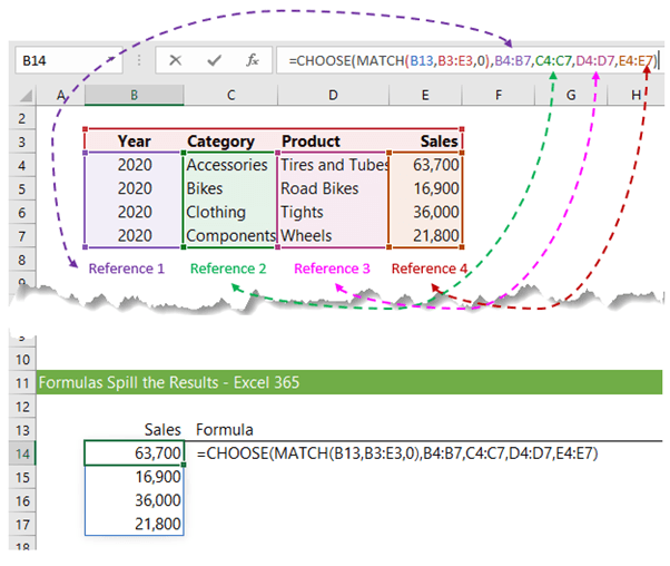
In the image below, cell B14 contains an OFFSET formula that returns the range E4:E7. The results spill to the cells below because I have Excel for Microsoft 365 and the new Dynamic Arrays, but essentially this formula returns a reference:

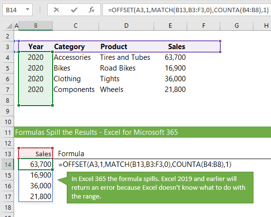
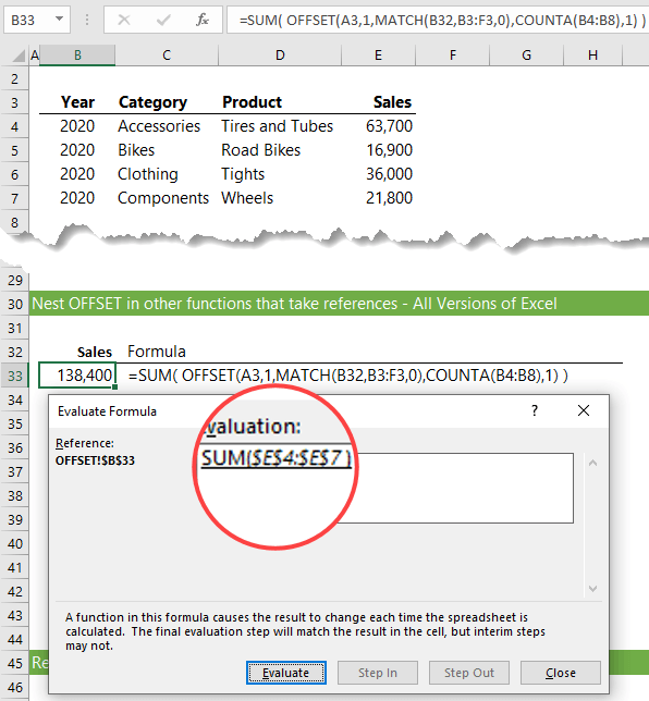
Earlier versions of Excel will return an error because Excel doesn’t know what to do with the reference returned. However, if we wrap the OFFSET formula in the SUM function it adds the values in the range E4:E7. And if you use the evaluate formula tool you can see the reference being returned, as shown below:

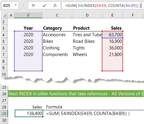
The above examples returned a single column however, you can also return rows, single cells or even a whole table (see example below). References to whole tables is useful for dynamic named ranges which can be referenced in formulas or as the source for PivotTables etc.

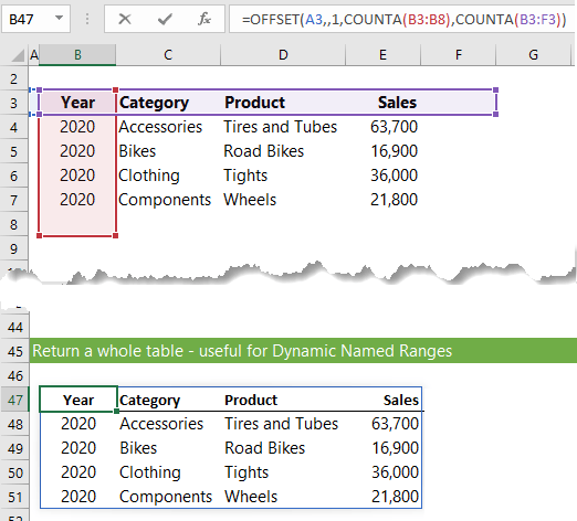
Notice the formula uses COUNTA to determine the height and the width of the table. The range in the COUNTA formulas reference an extra row and column to allow for growth in the table. In practice you would reference many more rows and/or columns in line with how much you expect the table to grow by.

OFFSET Pros

The biggest benefit to OFFSET is that it only takes one formula to return a reference to a single cell, column, row, or table.

We can easily determine a dynamic starting cell reference using the rows and cols arguments to find the starting cell for the range. e.g.

=OFFSET(A3,1,MATCH(B13,B3:E3,0),COUNTA(B4:B8),1)

Tells Excel to move one row down from A3 and use MATCH to find how many columns to move across to find the starting cell reference, which is E4. COUNTA then finds the end cell reference by counting how many cells high the range should be, which returns E7.

OFFSET Cons

It’s a volatile function, which means it recalculates every time a cell is edited and even in some other circumstances which can result in slow workbooks.

2. INDEX Function

Step by step tutorial on the INDEX function.

Syntax reminder:

=INDEX(array, row_num, [column_num])

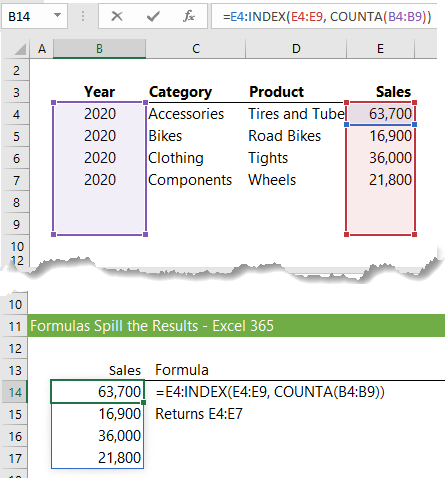
Like OFFSET, the INDEX function can also return a reference to a single column or row, or a whole table. The example below returns the reference to the Sales values in column E and you’ll see the approach is slightly different in that the starting cell, E4, is hard keyed in the formula before the colon operator and we only use INDEX to return the reference to the last cell in the range, E7:

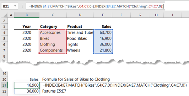
Note: We can use INDEX on both sides of the colon operator to return a range that has a dynamic starting and ending cell, as you can see below:

=INDEX(E4:E7,MATCH("Bikes",C4:C7,0)) : INDEX(E4:E7,MATCH("Clothing",C4:C7,0))

We can see in the image below that this formula returns the sales for Bikes through to Clothing:

Again, we can wrap the INDEX formula in SUM to add up the values in the range returned by INDEX:

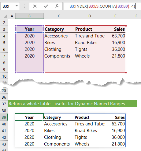
We can also return a whole table including the headers:

INDEX Pros

INDEX is non-volatile and far more efficient than OFFSET and INDIRECT, and it can return a reference to a single cell, column, row, or table.

INDEX Cons

If your reference also requires a dynamic starting cell reference, then you need to use INDEX on both sides of the colon

Note: When using INDEX on both sides of the colon operator it is always recalculated upon opening the workbook, which means it is momentarily volatile, but not once the initial recalculation has run. It’s still more efficient than OFFSET and INDIRECT

3. XLOOKUP Function (Excel for Microsoft 365 only)

Step by step tutorial on the XLOOKUP function.

Syntax reminder:

=XLOOKUP(lookup_value, lookup_array, return_array, [If_not_found], [match_mode], [search_mode])

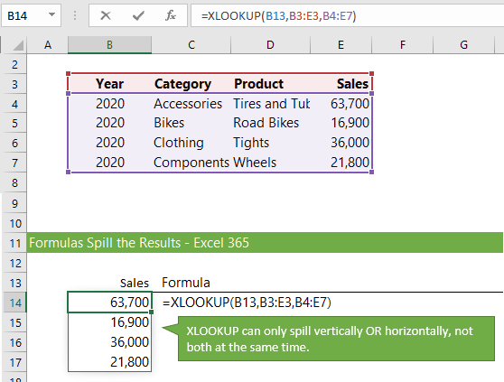
Unlike OFFSET and INDEX, XLOOKUP can only return a reference that is one column wide for vertical references, or one row high for horizontal references. In other words, XLOOKUP can’t return the reference to a whole table.

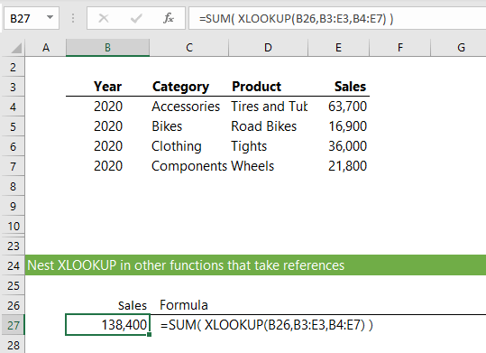
And of course, we can nest XLOOKUP inside of other functions that take references, like SUM:

XLOOKUP Pros

XLOOKUP is a much easier function to learn and use, plus it’s super efficient.

XLOOKUP Cons

XLOOKUP can only return a reference to a single cell, row or column, not a whole table consisting of multiple rows and columns. It’s also only available to Excel for Microsoft 365 users.

4. CHOOSE Function

Step by step tutorial on the CHOOSE function.

Syntax reminder:

=CHOOSE(index_num, value1, [value2],...)

With CHOOSE we can list several different references to ranges and with the first argument specify which reference to return. In the example below I’ve used the MATCH function to find the reference number for Sales:

Cell B13 (above) contains a data validation list that allows me to choose different references to return, as you can see below:

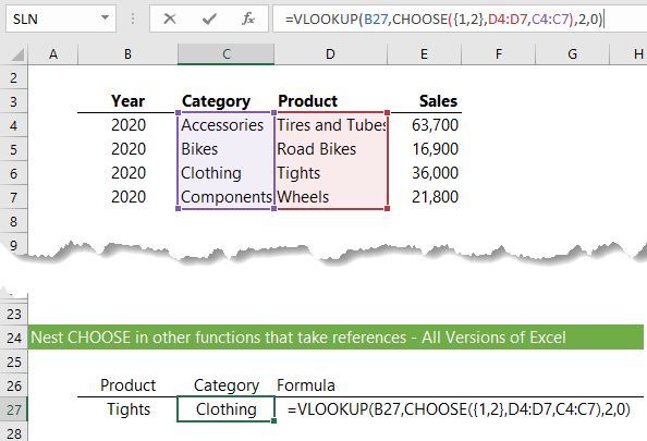
With CHOOSE we can also trick VLOOKUP into looking left by specifying which is column 1 and which is column 2. In the image below you can see that column D is listed first and column C is listed second. The array of {1,2} simply returns both references to VLOOKUP:

CHOOSE Pros

CHOOSE gives us the ability to rearrange the order of columns or rows and reference non-contiguous ranges, including references on other sheets.

CHOOSE Cons

CHOOSE on its own can’t return a dynamic range. You would need to also use another function, like OFFSET or INDEX in CHOOSE’s value arguments.

5. SWITCH Function (New in Excel 2019)

Step by step tutorial on the SWITCH function.

The SWITCH function is similar to CHOOSE, except is has a slightly different structure to its syntax.

Syntax reminder:

=SWITCH(expression, value1, result1, [default_or_value2], [result2],...)

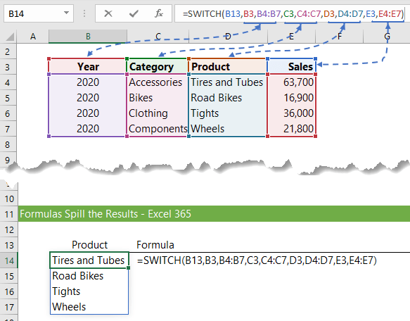
Again, you can link the expression argument to a cell containing a data validation list which allows the user to choose a different range to return.

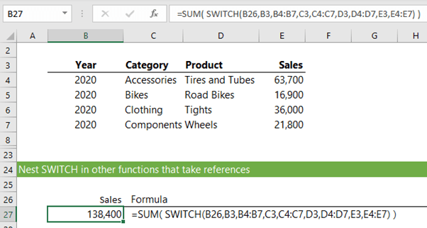
And you can wrap SWITCH in other functions that take references, like SUM:

SWITCH Pros

Those familiar with SWITCH from other programming languages will find this an easy function to use.

SWITCH Cons

Like CHOOSE, SWITCH on its own cannot return a dynamic range and it can’t return a reference to non-contiguous ranges.

6. IF Function

Step by step tutorial on the IF function.

Syntax reminder:

=IF(logical_test, value_if_true, [value_if_false])

We can replicate CHOOSE and SWITCH with nested IF functions:

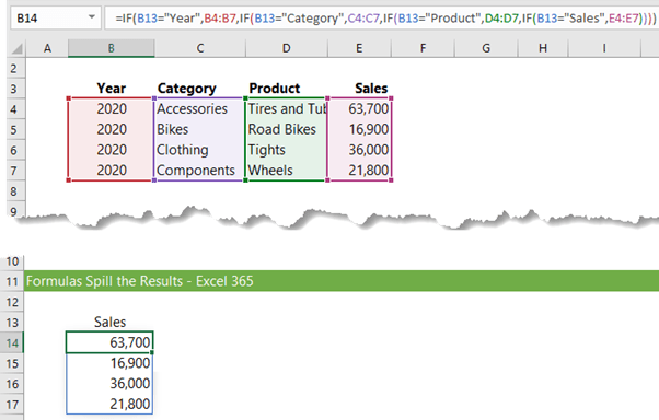
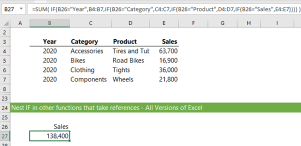
Again, users of Excel 2019 and earlier would need to either wrap the formula in another formula that uses the reference returned by IF, like SUM (shown below), or define a name.

IF Pros

IF has been around forever and many Excel users are already comfortable using it, which will make it easy to adopt for the use of returning references.

IF Cons

The IF function on its own cannot return a dynamic range. It’s not an efficient formula as each logical test will be calculated until a match is found, at which point it stops calculating. That said, if it’s not used in bulk then the calculation burden will be insignificant.

7. IFS Function (new Excel 2019)

Step by step tutorial on the IFS function.

If you have Excel 2019 or Excel for Microsoft 365, you can use IFS instead of having to nest IF formulas.

Syntax reminder:

=IFS(logical_test1, value_if_true1, [logical_test2], [value_if_true2]...)

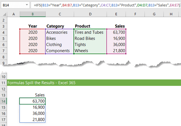
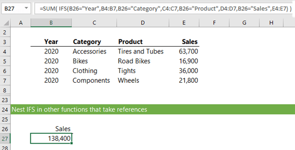
Like IF, IFS can be used in any formula that takes a reference:

IFS Pros

IFS is easier to write than a nested IF.

IFS Cons

Like IF, IFS cannot return a dynamic range on its own and will evaluate every logical test until one returns TRUE. As it’s only available in Excel 2019 onward, not many people will have access to it yet.

8. INDIRECT Function

Step by step tutorial on the INDIRECT function.

Syntax reminder:

=INDIRECT(ref_text, [a1])

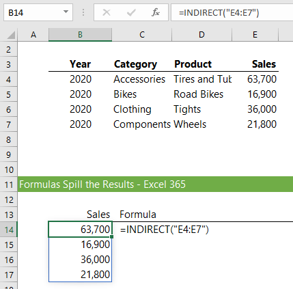
The INDIRECT function returns a reference specified by a text string as shown in the example below:

The cell reference text string can also be obtained by:

• referencing another cell, or
• generate it by nesting other functions

You can also use the ampersand (&) symbol to concatenate text and build a text string that way.

INDIRECT Pros

Probably the biggest positive for INDIRECT is that references hard keyed in the formula don’t update when rows/columns are inserted in the worksheet. E.g. =INDIRECT("E4:E7") will not change if a row is inserted above row 4 or to the left of column E.

Also, the reference can be built using text strings e.g. =INDIRECT("B27:B"&ROW(B35)) will return the reference B27:B35

INDIRECT Cons

INDIRECT is a volatile function and inefficient.

What about the FILTER Function?

You may be wondering about the FILTER function. After all, it spills the results like the examples above and can be nested inside functions like SUM and AVERAGE. However technically FILTER is not returning a reference.

This is best illustrated if you use the Evaluate Formula tool on any of the SUM examples above. You’ll see these nested formulas return cell references, but if you do this with FILTER it returns an array of values. And while this is fine for SUM, keep in mind that it won’t be any use if you wanted to use FILTER as a source for a PivotTable, as this requires a reference.

The Best Excel Function that Returns a Reference

With 8 different functions that can return references, you’re probably wondering which one is best.

There isn’t one that’s best, but if you want to return a reference to a table, I’d use INDEX because it’s not volatile like OFFSET.

If you need to return a reference to non-contiguous cells or you want to rearrange the order of columns or rows, then use CHOOSE.

And if you only need a single column or row of cells, then XLOOKUP is super easy to use and very efficient for Excel to calculate.