5 Excel INDEX Function Secrets

The Excel INDEX function is a treasure trove of functionality, but most of us only know one way to use it. In this post I want to expose some lesser known quirks and ways it can be used.

 

1. If the reference/array is a single row, you can put the col_num in the row_num argument’s position
2. INDEX can return a cell or range reference
3. 0 or skipping the row/column argument will return the whole row/column
4. INDEX can be used either side of the colon, space or comma operators
5. INDEX can return non-contiguous areas

Let’s start by quickly revisiting the syntax for the INDEX function. It has two syntax options:

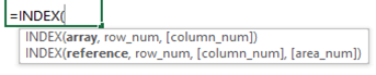
The first version takes an array of values, and the other takes a reference to a cell, or range of cells. You don’t choose which syntax to use, Excel will decide that based on the inputs.

The output can be a single value, an array of values or a reference to a cell or range of cells. The output will depend on the context of the formula. For example, whether the formula is entered in a single cell, nested inside another function, array entered etc.

Watch the Excel INDEX Function Video

Download the Excel INDEX Function Workbook

1. Use row_num for col_num when reference/array is a single row

The formula in cell C16 looks up cells C7:F7 i.e. a row and returns the value from column number 2.

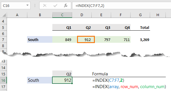
Remember the syntax for the INDEX function relevant to this example is:

=INDEX(array, row_num, [column_num])

And the formula above is:

=INDEX(C7:F7,2)

Notice the col_num argument is in the row_num argument’s position. When the reference is a single row, you can simply specify the column number in the row_num argument.

2. INDEX Function Can Return a Reference

The formula in cell C16 below looks up the value for West, which is in row 4 and Q2 which is in column 2:

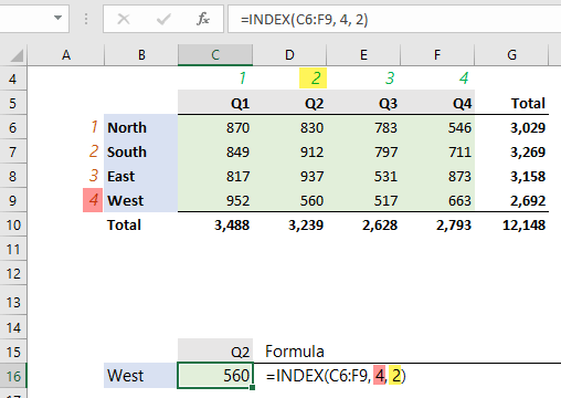
Note: Most of us would use INDEX with MATCH to return the row_num and column_num arguments, but I want to keep this simple for the next example.

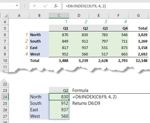
Depending on the formula, the return value of INDEX may be a value, as we saw in the previous examples, or a cell or range reference. In cell C24 (image below) INDEX returns a cell reference, D9, and because I have dynamic arrays, the results spill to the cells below:

Excel 2019 and Earlier Notes:

1. If you have Excel 2019 or earlier, you first select 4 cells, then enter the formula by pressing CTRL+SHIFT+ENTER.
2. If you entered the formula in Excel 2019 or earlier without pressing CTRL+SHIFT+ENTER, Excel would only show you the first result i.e. 830 because it wouldn’t have enough cells to display all the results returned by the formula.

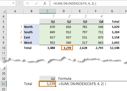
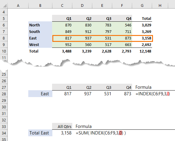
If you wrap the above formula in SUM (in any version of Excel) it will add the 4 cells like so:

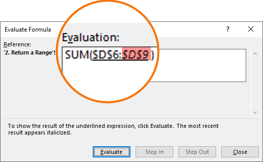
We can see INDEX evaluates to a cell reference in the Evaluate Formula dialog box:

3. Return a Whole Column or Row

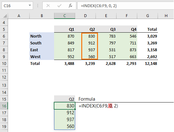
If you place a zero in or omit the row_num or column_num arguments, INDEX will return the whole column or row, respectively.

In the example below in cell C16 you can see the row_num argument is zero, and INDEX has spilled the results of the whole column (D6:D9) to the cells below:

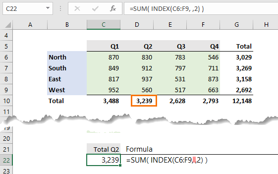
Similarly, in the formula below, the row_num argument has been omitted, and again INDEX returns the whole column, which is then summed to return the total, 3,239:

The same rule applies with the column_num argument as you can see in the examples below:

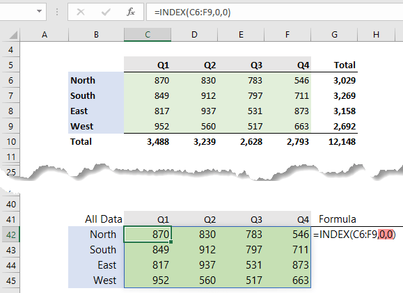
Of course, zeros in both the row and column numbers or omitting these arguments altogether will return the whole range specified in the array/reference argument:

4. Operators

In example 2 we saw INDEX return a cell reference. This ability makes it perfect for returning dynamic named ranges. And if you know me then you’ll probably have seen me use INDEX for this before.

Colon Range Operator

The INDEX function can sit either side of the colon operator like so:

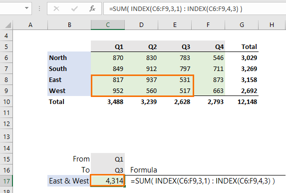
When teamed up with MATCH (see below) it can return a dynamic range that can adapt to changes in the selected quarters in cells C15 and C16:

=SUM( INDEX(C6:F9,3, MATCH(C15,C5:F5,0) ) : INDEX(C6:F9,4, MATCH(C16,C5:F5,0) ) )

Comma Union Operator

INDEX can also be used either side of the union operator, the comma. In the example below it is used to return two quarters, which are then summed:

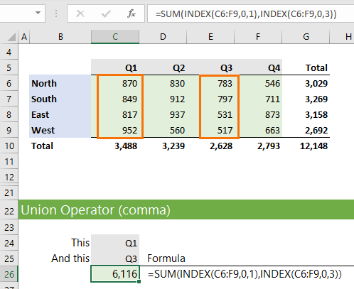
When MATCH replaces the hard-keyed column references, it becomes dynamic:

=SUM(INDEX(C6:F9,0,MATCH(C24,C5:F5,0)),INDEX(C6:F9,0,MATCH(C25,C5:F5,0)))

Space Intersect Operator

The intersect operator returns the value at the intersection of two ranges.

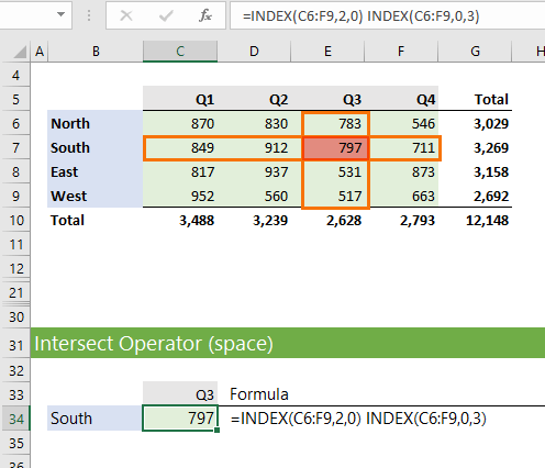
Again, we can team INDEX with MATCH to make the formula dynamic:

=INDEX(C6:F9,MATCH(B34,B6:B9,0),0) INDEX(C6:F9,0,MATCH(C33,C5:F5,0))

5. Non-contiguous Ranges

The less commonly used area_num argument allows you to reference multiple non-contiguous ranges. The references to the ranges are wrapped in parentheses and separated by a comma. I’ve named the ranges Product1 (C6:F9) and Product2 (H6:K9):

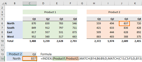
The areas are numbered in the order you enter them, so in this example, product 1 is the first area and product 2 is the second area.

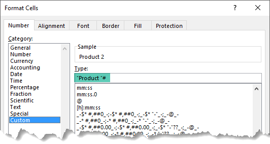
Note: Cell B13 contains the area_num. I’ve formatted it with a custom number format so that the text, ‘Product’, prefixes the number. You can see the format in the dialog box image below:

Notes:

1. The area ranges must be on the same sheet, otherwise INDEX will return the #VALUE! error.
2. The area ranges don’t need to be the same size, however it they aren’t it will be tricky to choose the correct row or column as it’s expected the structure of the tables is the same.