The Excel VLOOKUP formula is my favourite! Perhaps because it was one of the first formulas I mastered. It gave me an insight into the power of Excel and how it could help me in my job.
Interestingly, there are two ways you can use the VLOOKUP function; exact match and approximate match. However, I find that most people know one way or the other, and only a few know both.
Excel VLOOKUP Formula Video Tutorial

Download the Workbook
Enter your email address below to download the sample workbook.

Excel VLOOKUP Formula Written Example
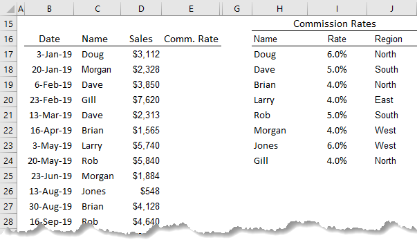
Using the example data below, I want to lookup the commission rate in column I of the table that's in columns H:J, for the salesperson listed in column C, and put the result in column E.
Excel VLOOKUP Function Syntax
Before we get started, let's understand the VLOOKUP function's syntax.
=VLOOKUP(lookup_value, table_array, col_index_num ,range_lookup)
And to translate it into English it would read:
=VLOOKUP(find this value, in that table, return the value in the nth column of the table, but only return a result if you can match the value exactly*)
* for an exact match you must specify FALSE or 0 in the last argument of the VLOOKUP formula.
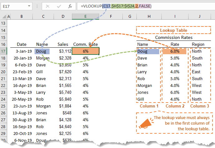
Let’s make it even clearer by applying it to our example:
=VLOOKUP(find the name Doug from cell C17, in the Commission Rates table H17:J24, return the value in column 2 of the table, but only return a value if you find the exact name "Doug" in the Commission Rates table, otherwise give me an error)
Rules, Common Mistakes and Troubleshooting!
- ‘Return the value in column 2 of the table’ is referring to the column number in the table H17:J24, not the column number of the spreadsheet. The information we want returned is the percentage rate, and it is in the second column of the Commission Rates table.
- ‘Only return a result if you can match the value exactly’ is telling Excel that we only want information returned if it matches our criteria exactly. i.e. Find Doug in our Commission Rates Table, and if you can’t find Doug, give me an error. The error displayed will be #N/A.
- VLOOKUP formulas read from left to right. You must have the information you are looking up (in our example the salesperson's name), in the first column of the lookup_array range.
- Lookup Table Location: The ‘Table’ you are looking up can be in the same spreadsheet. Or a different sheet in the same workbook. Or in a different workbook altogether.
- Sort Order: The table doesn’t have to be sorted in any particular order when using the Exact Match version of the formula, but you must not have duplicates. Unless the information on each duplicate is exactly the same. For example, if Doug appeared twice in our Commission Rates table with different percentage rates for each instance, VLOOKUP would return the rate on the first instance of Doug.
- VLOOKUP isn't case sensitive, so 'Doug' could be 'doug' or 'DOUG' or 'Doug', in either column C or the Commission Rates table.
When VLOOKUP formulas return #N/A errors it means Excel can't find the value you're trying to look up in your table. If you get this, but you can ‘plain as day’ see it's there in the table, then it’s likely you’ve got one of the values prefixed with an apostrophe. To check this go to each cell you're referencing and look in the formula bar and see if there is an apostrophe in either cell. You can only see the apostrophe from the formula bar. See example below.
Text Formats: Excel reads text prefixed with an apostrophe different to text without. Even though on the face of the spreadsheet they might look the same. You need to make sure both the value you're looking up, and the value in the table either both have the apostrophe, or both don't. The quickest way to get rid of the apostrophes is to do ‘Text to Columns’. Or run it through the VALUE function, which converts numbers formatted as text to actual numbers.
- Leading or Trailing spaces are another cause of VLOOKUP errors. Edit the cells to check if there are extra spaces before or after the lookup value, or the data in the first column of the lookup_array. Use the TRIM function to easily clean leading and trailing spaces.
- Dynamic Column References: Use COLUMNS or the MATCH function to dynamically find the col_index_num argument for VLOOKUP. See the video above for step by step instructions.

Excel VLOOKUP Approximate Match Formula
Now you've mastered the VLOOKUP exact match formula, you're ready to learn VLOOKUP approximate match. This technique is lesser known and many people make the mistake of using a nested IF formula instead of this simple approach.


Sometimes I write one formula and this not give me back de solution value. Only show de formula instead of the solucion of the operation.
I do not know why.
It’ll be because the cell is formatted to Text before you enter the formula. Sometimes cells will automatically copy down formatting from the cell above.
Good morning from Nigeria i will like the pdf explanation on on all the lookups i will be glad if my request is granted thanks God Bless.
There’s not enough information. Please post your question on our Excel forum where you can also upload a sample file and we can help you further.
Hi,
I’m afraid we don’t have any PDF explanations for the lookup functions. But you can search our blog for the term lookup and you’ll find lots of posts.
Or you can take our Advanced Excel Formulas course
Regards
Phil
INDEX where in the row MATCH Sheet1 D7(date) in Sheet2 E:E and match Sheet1 F1 in any one cell Sheet2 B2 to U2 (sheet 1 F$1 equal to all the cells in Sheet2 from B2 to U2-any code number), and match Sheet1 G$1(text) in only one cell in Sheet 2 B4 To U4. next Sheet1 D8 for entire column
Hi Sudha, please post your question on our Excel forum where you can also upload a sample file and we can help you further.
How do i use vlookup formula to below
Agent ID Remaining Leaves Bonus
2345 6 2000
5457 4 3000
9823 7 4000
1233 2 3000
2344 8 5000
You’ve been asked to come up with a way to check the bonus of the agent when the Agent ID is typed into a given cell
Agent ID 2344
Bonus
Hi Ruby,
This looks like a test question. There is some information missing, namely how the bonus is calculated. However, you might find this VLOOKUP on a sorted list helpful.
Mynda
I am trying to use this =VLOOKUP($A4,Data2!$A:$AC,H$1,FALSE) to pull forecast for multiple months from data file but this does seems to be working, could you please walk me through to use this formula appropriately ?
There’s nothing obvious wrong with your formula, so it must be an issue with the data in the cells being referenced. You can post your question on our Excel forum where you can also upload a sample file and we can help you further
How do I set up a formula for removing a list of names in sheet 1 from a larger list of names in list 2 and thus, have fewer names in list 2 with none of the names as per list 1?
Hi Gabriel, you can use Power Query to compare the lists.
After struggling with VLOOKUPS for days, this has been the clearest explanation I’ve seen of how they work. After reading this guide (especially the part where you applied it to your example), I was able to do my VLOOKUPS in no time. Thank you!
So pleased I could help, Lauren!
this is description also available in another language ? like us (hindi)
Sorry, Kamal, we don’t have it in other languages.
its ok thanks for you
Please help me understand each of the arguments in this lookup formula:
=LOOKUP(1,1/($A$5:$I$5″”),$A$5:$I$5)
What does the “/” character do?
Changing the number in the first argument doesn’t seem to effect the result. Why?
I can utilize the formula but would like to understand it.
Hi,
That is not a valid formula. Please see LOOKUP Function
The set of double quotes should not be there and you are using the same range for the lookup vector and the result vector. Something like this would work
=LOOKUP(1,1/($A$5:$I$5),$A$6:$I$6)
Where
A5:I5 is 1, 2, 3, 4, 5, 6, 7, 8
and
A6:I6 is a, b, c, d, e, f, g, h, i
The input vector is therefore 1/$A$5:$I$5 i.e. 1/2, 1/3, 1/4, 1/5 etc
Changing the first argument (the lookup value) can affect the result but it will depend on what your input vector and result vector values are. If the first argument is not found, the result is the smallest value nearest the lookup value. Unless the lookup value is smaller than the smallest value in the lookup vector, in which case you’ll get an error.
Regards
Phil
Phil, Thank you for your prompt reply. There was a typo in the formula I presented.
The goal was to lookup the last non-blank entry in a designated range and then return the corresponding entry in a second designated range.
My corrected formula should read:
=LOOKUP(1,1/(A8:I8<>""),A14:I14) This worked for me but I wanted to understand the arguments.
It seems to count over to the last non-blank entry in row 8 and then returns the corresponding entry in the (same column) second designated range. (in this formula (A14:I14). If the “” expression is omitted, the result vector is offset by – I wish to understand exactly what each argument does – specifically, the first and second arguments and the “/” character and how to offset the result vector.
Your assistance is much appreciated.
Hi Harriman,
To check for the last non-blank entry you need to use 2 as your lookup value i.e.
=LOOKUP(2,1/(A8:I8<>""),A14:I14)
Let’s say A8:I8 contains a, b, c, d, e, f, g, h, i
and A14:I14 contains 1, 2, 3, 4, 5, 6, 7, 8, 9
(A8:I8<>"") gives an input vector of True or False values depending on whether or not the cell contains a value or to be more specific does not contain a null string.
You get {True, True, True, True, True, True, True, True, True}
If A8:I8 contained a, b, c, , e, f, g, h,
then your input vector is {True, True, True, False, True, True, True, True, False}
Dividing 1 by this vector
1/{True, True, True, False, True, True, True, True, False}
gives you
{1, 1, 1, 0, 1, 1, 1, 1, 0}
Actually 1/False gives a #DIV/0 error but let’s call it 0 as it works the same way here.
The way LOOKUP works is to return the lookup value or if that is not found, it returns the nearest smaller value.
By using 2 as the lookup value, LOOKUP works through the lookup vector for 2 but can’t find it, so it returns the position of the last 1, which in ths example is position 8.
So you get 8 returned from the result vector.
If you need more help please start a forum topic so I can send you a workbook with an example of this.
Regards
Phil
Hi please explain vlookup multiple sheets foumula in cleary
You can see a tutorial for VLOOKUP multiple sheets here.
Thank you for your great offer
Hello , i shoud do an invoice and i must use vlookup formula and i dont know how to do exactly…i must multiply 10*(0.01*2) can you help me please?
Hi Bogdan,
I’m not sure why you need a VLOOKUP to multiply numbers ?
Can you please start a topic on the forum and supply your workbook so we can better understand what you need.
Regards
Phil
Hi Myrnda,
I have an excel file with two sheets in two tables.
Table 1 – having a cost center and cost spread across 12 columns.
Table 2 – Having the same cost centers and would like to use the vlookup formula to populate the data from Table 1 without having to change the column reference for each of the 12 columns.
I did try the formula in the article but it does not work and I get an error message.
Is there a different formula is using this formula for more than one sheet or am I making a mistake?
Your help would be much appreciated.
Regards, Ramki
Hi Ramki,
You can use the COLUMN Function to dynamically update the column number argument in VLOOKUP like so:
Assuming the first column you want returned form the table_array is 2.
If that doesn’t help, or if you still have questions please post your question and sample Excel file on our forum where we can give you a specific answer.
Mynda
i have really enjoyed it
Great to know, Zacharie!
Thank you – this was helped me get through a bit of a brain-fart moment… lol. Good article!!
🙂 glad it was helpful.
Thank you.
Nice tutorial
Thx Ginta
ohhh i love this….. i have my igcse in two days and this really helped me out
Glad you found it helpful. All the best with your igcse!
My vlookup will not copy correctly. I have the calculations function set to automatic. I have all the references except the column number as absolute but it stilll produces the exact same answer instead of moving across a formula. Any suggestions why?
Hi Christina,
Hard to tell without seeing the formula and workbook. Can you please post your question and Excel file on our forum where we can help you further.
Mynda
Nicely done.
Cheers, Michael 🙂
Super cool.
Super awesome..
Thanks! Glad I could help!
I absolutely love your videos and how you clarify steps and what the formulas mean and what they are extracting. I have watched MANY training videos and yours are the best! THANK YOU!
Aw, thanks Julie 🙂 Glad you enjoyed them.
Mynda
Same with me I feel it is the best.
Thanks, Amani 🙂 Great to know I can help.
Well explained.
Thanks, Naveed 🙂
Hi Sir ji Please help me
if one row lots of code 41 or 37 etc and next row lots of grade A1, A2, B1 i want to know how many code 41 get A1 or how many 37 code A1 what formula used. show below chart what formula use it.
SUB MRK GRD SUB
41 88 A2 42
37 99 A1 42
41 78 B1 42
37 94 A1 42
41 64 B2 42
41 59 C1 42
41 79 B1 42
41 33 D2 42
41 95 A1 42
42 65 B2 43
Advance Thanks
Have you tried the formula you already have?
=SUMPRODUCT(($A$2:$A$12=37)*($C$2:$C$12=”A1“))
=SUMPRODUCT(($A$2:$A$12=41)*($C$2:$C$12=”A1“))
Catalin
Thanks a lot for the ebook Tips & Tricks. Unfortunately, it’s not as what I wanted. I am looking for help to do with lookup database pictures. The result from vlookup data from the table as the result should be picture as wanted. Although, I have some examples from the internet but Sorry I’m not satisfied with them. I hope might be you would help me, please. Thanks a lot.
Hi Emmanuel,
Can you please provide a sample file and detailed descriptions for what you are trying to achieve? You can use our Help Desk System to upload the file, please create a new ticket.
Cheers,
Catalin
Hi.. Pl help me identifying the 1st , 2nd and 3rd max values from an array…
ex:
Array
Project Version
A 13
A 3
A 4
A 2
A 5
A 8
A 18
A 11
A 7
A 23
A 24
A 6
A 12
A 1
A 9
B 5
B 2
B 3
B 1
B 6
B 4
I want the 1st , 2nd and 3rd max values of project ‘A’ in the cells z1, z2, & z3, likewise for project ‘B’ in y1, y2 & y3…
Pl help…
thx
Kamal
Hi Kamal,
You can use this formula in Z1, and copy it down to Z3:
=LARGE(IF($A$1:$A$21=”A”,$B$1:$B$21,0),ROW(A1)) entered with Ctrl+Shift+Enter (it’s an array formula)
For largest B projects: use this formula in Y1, copied to Y3:
=LARGE(IF($A$1:$A$21=”B”,$B$1:$B$21,””),ROW(A1)) entered with Ctrl+Shift+Enter (it’s an array formula)
Cheers,
Catalin
Hi Catalin… It works for me… Thanks very much… Just now I m hearing about array formula.. if you have notes on that, pl share…
Now I have another request… its continuation of my earlier request…
Project sub-proj Version
A qwe 13
A rty 3
A uio 4
A plk 2
A jhg 5
A fds 8
A azx 18
A cvb 11
A nml 7
A kjh 23
A gfd 24
A saq 6
A wer 12
A tyu 1
A iop 9
B mnb 5
B vcx 2
B zas 3
B dfg 1
B hjk 6
B lop 4
I want the sub-proj name of 1st , 2nd and 3rd max values of project ‘A’ in the cells z1, z2, & z3, likewise for project ‘B’ in y1, y2 & y3…
pl help…
Thx
Kamal
Hi Kamal,
Please describe from the beginning the entire problem, because any little detail can change the approach, and the solution may be totally different.
Try this file from our OneDrive folder. The solution works fine if you do not have duplicates, at least for the highest 3 numbers.
Cheers,
Catalin
Pl let me know, how to share my xl sheet
Hi Kamalnath,
You can send it to us via the Help Desk.
Cheers,
Mynda
Madam, I find the tuitorial guide very helpful. Would you please explain to me how we proceed with VLOOKUP using multiples sheet.
Thanking you
Kumar
Thanks, Kumar.
You can see the VLOOKUP for multiple sheets tutorial here:
https://www.myonlinetraininghub.com/excel-vlookup-multiple-sheets
Kind regards,
Mynda
Learn far from here
Thanks, Peik 🙂
Hello MEL
Yes their are very lively presentations are excellent and make Excel be simple.
Hi Mynda, I am trying to do some analysis on a s/s. I have a worksheet which has data arranged in columns, such as instance, location, months. I have another s/s with new data for the current month. I am trying to compare data from the current month to the existing s/s and if data (instance and locations) match, then add this new data as a new column to the existing s/s. The instances column should have unique data, but if there are data in the new or existing s/s that do not match, then append them at the bottom of the existing s/s. What formula should I use? Thanks for your help.
Hi Mel,
I hate to say this but I think your approach isn’t ideal. There is no easy way to do what you describe using formulas… or any other Excel tool.
Perhaps if you can send me your workbook I can better understand what you’re trying to do and give you some advice on how to acheive the same end result with some changes to your process.
You can send your file and description of what you want and where via our help desk – anything you send is kept confidential.
In the meantime you might find this tutorial on Tabular Data helpful.
Kind regards,
Mynda
got gd
Very useful material.
Glad we could help, Ranjha 🙂
hi can you please sent me a emaill and explean the why we use the VLOOKUP AND ALSO EXPLAN AS WELL THANKS A LOT PLEASE
Hi,
VLOOKUP is an Excel Function that is used within tables to help filter through large volumes of data and
select the appropriate data based on given conditions. The VLOOKUP formula would automatically look through the list of your Objects and pick out
the corresponding data.
The function is very well described in this tutorial , please take your time to understand the explanations, you can also download an example workbook, the link for download is at the end of the tutorial.
Catalin
Wonderful, I need some more examples to master this formula. i would also like to learn about sub total.
Thanks
Thanks, Yogi. If you mean the SUBTOTAL Function you can learn it here.
Otherwise, a tutorial on the Subtotal tool is here.
Cheers,
Mynda.
Nice information….
Thank you, Harish 🙂
Loved it. Nice and simple and that “plain english” translation is just superb !!!!
Thanks, P. Glad you found it useful 🙂
by v look up the answer comes only up in the function arguments but in the cell only coming up v look up (example) but not the answer
Sorry, Sim. I don’t understand. Can you please give me an example?
Cheers,
Mynda.
Sir,
In my Laptop Excel sheet’s are viewing as for Rows 1,2,3,… are making visible and for coloums 1,2,3….. are visibling insted of A,B,C… how to chage it?
Hi BNS,
You’ve got R1C1 reference style turned on. To turn it off you need to access the Options (Office button for 2007 or File tab for 2010) > Formulas category > uncheck ‘R1C1 reference style’.
Kind regards,
Mynda.
Can solve this puzzle from a spread sheet from 1996 deals with gas processing Question on VLOOKUP Function This is part of a spread sheet
Amine Treater
Amine type (MEA, DEA, MDEA) DEA Typical Amine solution properties are shown below:
Many cells left out
Amine Properties Lookup Table
Amine Wt% Loading SG @ 120F Mole Wt BTU/Gal
MEA 15 0.33 0.99 61.08 1200
DGA 50 0.35 1.058 105.14 1300
DEA 30 0.35 1.02 105.14 1100
MDEA 50 0.35 1.03 119.16 1000
Intermediate Calculation Results
CO2 and H2S to be removed 60.84 lb-moles/hr
Solution specific gravity 1.04 VLOOKUP(UPPER($C$27),PROP,4,FALSE)
Amine molecular weight 105.14 =VLOOKUP(UPPER($C$27),PROP,5,FALSE) Do you know how cell DEA($C$27) at the top of the sheet is referenced to the two cells for Specific Gravity 1.04 & Molecular Weight 105.14 is nested or referenced?
Can’t find the chart UPPER on the spread sheet. PROP is Amine Look Up Table, immediately above the text.
Could send he spread sheet to you.
Regards….
Hi Charles,
I think it’s best if you send me the Excel file so I can see what you’re talking about.
Cheers,
Mynda.
It is very helpful website I have ever visited. I recommended already to all of my friends and the love it.
Thanks, Ateny 🙂
Great!
I got a format from a resigned employee, but I don’t understand “,IF({1,0},…”, I cannot find information why there is {1,0} in the IF.
=VLOOKUP(B2&E2,IF({1,0},’PT New Sales’!$C$2:$C$200&’PT New Sales’!$F$2:$F$200,’PT New Sales’!$G$2:$G$200),2,FALSE)
Please help, Thanks
Hi David T,
In the IF({1,0} the 1 = TRUE and the 0 = FALSE.
The formula is testing to see if the value in B2 is in the range C2:C200, and if the value in E2 is in the range F2:F200, if both match return the value in column G.
It’s an interesting formula. I have not seen it done this way before. I hope that helps.
Kind regards,
Mynda.
P.S. I have to thank Roberto Mensa for helping me clarify what this formula is doing 🙂
You bring clarity to Excel. I am not just applying a formula, now I know what each component parts mean.
Thank you
Barb
That’s my pleasure, Barb 🙂
S..really it’s a great job.
Cheers, Ramkumar 🙂
It is very useful,thanks for that,but i want to ask,if Commissioning rates(As per example) is another excel sheet,so can we use vlookup,I tried but is showing error?
Hi Yash,
Please send your file here HELP DESK.\
I just want to see why it’s an error and how you did it.
Cheers,
CarloE
Firstly thanks for an awesome site. I have intermediate excel skills, but you’re explanations have made learning new formulas really easy!
In relation to VLOOKUP – I’m using it in a training register to confirm who has completed which training on what date. The column with the formula is formatted for dates as dd/mm/yyyy. Some people haven’t completed the training yet, and rather than leaving the cell blank it gives the result 0/01/1900. This is the formula as I’ve put it in the sheet =VLOOKUP($A5,Induction!$A:$C,3,FALSE). Is there any thing I can do to make it leave the cell blank if the reference is blank or perhaps a different formula I could use
Hi Penelope,
All you need to do is put it inside an IF function like this:
More IFs
Cheers,
CarloE
Thanks heaps for that CarloE 🙂
Hi Penelope,
My pleasure.
Cheers,
CarloE
Dear,
I need a help with Excel formula, probably it’s easy but I can’t get it!
I have a table of one month and in 2right columns 2 figures, the form is used for account.
I made a box with Now() and want to make a formula to take data from table for present day. So first have to confirm same date as today from table and then to take data from 2right columns.
Thank You Very Much in Advance
Pero
Hi Pero,
Please send your file via help desk. and we can look at this for you.
Cheers,
Carlo
I downloaded the Excel workbook excercises (https://www.myonlinetraininghub.com/excel-2007-%e2%80%93-vlookup-formulas-explained) but they would not open in Excel. It would be appreciated if you can help me to overcome this problem.
Thank you for your help.
Arvind
Hi Arvind,
I would say either your browser has changed the file extension of the workbook from .xlsx to something else, or you are using Excel version pre-2007?
You can try again and make sure the file extension is .xlsx of the saved file.
If you have Excel 2003 or earlier let us know and we’ll make a pre-2007 version available.
Cheers.
CarloE
hi mynda,
can u help me in vlookup formula.i think it is scarry for how use this formula in very easy.i have two difrent sheet in two difrent file .tell me how can i handle this…………plzzzzzzzzzzzzz
Hi Hassan,
Here’s an example. I want to lookup Aquino, Greg’s position in Sheet2
The Formula:
Data:
Workbook1:Sheet1
      A                   B
1 Aquino, Greg	[VLOOKUP FORMULA HERE]Pitcher
Workbook2: Sheet1
Read More: VLOOKUP
Cheers.
CarloE
If some time invest the amt 12000 in medicine and after the selling received total amt 18000 , how many % income
Hi Manoj,
It’s a simple formula.
Data:
Formula:
I hope it helps.
Cheers.
CarloE
Hi Mynda!
We can use Vlookup either side…
=VLOOKUP(E2,CHOOSE({1,2},$B$2:$B$13,$A$2:$A$13),2,FALSE)
=VLOOKUP(CRITERIA,CHOOSE({1,2},CRITERIA RANGE,LOOKUP RANGE),COLUMN NUMBER,FALSE)
Hi Proficient,
Thanks for sharing.
You may also read our similar post here: VLOOKUP and CHOOSE
Cheers.
CarloE
Many Thanks..
Cheers, Jasim. You’re welcome 🙂
Hi
I have two tables one with colum name as “login id” and another with “computer name” and same colum in other sheet. i just want to compair login id and copy respective computer name to it. i tryed following funtion
=VLOOKUP(A2,sheet2!A:b,2,0) result is #N/A
Hi Mohammed Adil,
Your VLookup should look like this:
Your Table Array part don’t have the row arguments. It must have the numbers in other words i.e. Shee2!A2:B4.
Read more on VLOOKUP BASICS
Sincerely,
CarloE
I have used this lookup formula for years with complete confidence.
=if(vlookup(cell,range,1)=cell,vlookup(cell,range,Column # to be returned),” “). This returns an exact match if found and a blank cell if not.
But I have run into a problem, my formula is not returning anything on some newly added items in the lookup range. The item are still in sorted order and still in the lookup range. The format of the information is a match. Have you come across this?
Hi Lynn,
Please try to send your file through HELP DESK so we can have a good look at your problem.
Anyways, my diagnosis is that you did not have absolute references to your table_array part
of your VLOOKUP.
For example
You can do this by highlighting the ranges -only i.e. C5:D9- and press F4; or
You can simply put Dollar($) sign manually.
Cheers.
CarloE
Hi Mynda. The best for you in 2013… As usual, finding the best answers here… Excellent job, really.
Mynda, I’m having a trouble. Your explanation was great on the Vlookup formula syntaxis, but I was just wondering if the “col_index_num” requirement would look into rows instead of columns…. How would achieve that? I guess this function isn’t going to work for me, since I need to return a value that’s five rows under the respective “lookup_value” reference, and not to the side…
Is there an equivalent to this formula, but reading from the top of a table to its bottom?
=VLOOKUP(lookup_value, table_array, col_index_num ,range_lookup)
Hi Mynda. I guess I found it and did it, using the HLOOKUP function that you also explained here in the blog (sorry):
=HLOOKUP(AOR35,AK4:BG9,6,FALSE)
Thank you very much for your lessons.
Hi 6tel,
Happy New Year to you too 🙂 Glad you found the HLOOKUP solution.
Kind regards,
Mynda.
is very yousfull my life in my care
NICE WAY OF PRESENTING THAT’S TO EXLPNATION IN ENGLISH I.E –
And to translate it into English it would read:
VLOOKUP(find this value, in that table, return the value in column x of the table, but only return a result if you can match the value exactly)
VERY SUPERB
TNK U
Thanks, Sreedhara 🙂
How to search multiple entries by using Vlookup
Hi Reeta,
Here is a tutorial on VLOOKUP multiple values.
If that’s not what you want there is a list of different VLOOKUP tutorials here, including multiple criteria, multiple columns and returning multiple values.
Kind regards,
Mynda.
Excellent way of explaining. Easy to understand
Thanks, Viswanathan 🙂
Great help for searchers like me. Thanks a ton..
You’re welcome, Devikarani 🙂
I have a challenging excel vlookup problem I can’t solve and I can relate it to your example.
In my problem there is an additional column in the table of rates called “effective date”.
Insert a new column between Column G:H, and add title “Effective Date” Then give all those in your rates table an effective date of 01 Jan 08.
However, Dave gets a raise on 01 Mar 08 to 6% commission. (Well done Dave!)
Insert a new entry below Dave’s 01 Jan 08 entry and add:
01 Mar 08 Dave 6%
However, with your current formula, it does not find Dave’s new rate for sales after 01 Mar 08.
I have tried index match formula’s but also to no avail.
I really, really, hope you’re able to help as this has been bugging me for months.
Many thanks for your time. Regards, Martin
Hi Martin,
If you know you are looking for the date on 01 Mar 08 you could use SUMIFS:
or if you’re using Excel 2003 use SUMPRODUCT:
=SUMPRODUCT((I5:I6)*(G5:G6="Dave")*(H5:H6=DATEVALUE("01/03/2008")))However, if you’re just looking for the last record for Dave (your data would need to be sorted in ascending order) then you can use:
=VLOOKUP("Dave",$G$5:$I$6,3,TRUE)or
=LOOKUP("Dave",$G$5:$G$6,$I$5:$I$6)Where column G contains your names, H your dates and I contains your commission rates.
Kind regards,
Mynda.
Thanks for the prompt reponse and the numerous solutions.
I’ll try those out and see if I can get them to fit my situation.
Again, many thanks, your prompt response has been much appreciated. 🙂
Finally found a clear explanation in plain english on how to use this function. Wish i had found this site 1 hour ago! Thanks!
🙂 Thanks, Garth.
i want to know about pivot table in Excel 2007
Here’s a link to some tutorials on Pivot Tables https://www.myonlinetraininghub.com/pivot-table
Phil
Here we’re doing VLOOKUP in same worksheet,
can you give me VLOOKUP formula using different worksheet.
Hi Prakash,
When you build your VLOOKUP formula you can use your mouse to select the cells on another worksheet. Excel will automatically put in the cell references for you.
Kind regards,
Mynda.
Great tutorials – thankyou for sharing your knowledge. Greatly helped me in my work.
You’re welcome, Trudi 🙂
Nice. I especially like the extending of the VLOOKUP to do calculating.
Cheers, Steven 🙂
Finally. I have found someone that can translate “computer lingo” into English.
I have been lost in the land of technology, and then……. I have found my little slice of heaven. This website.
From one bean counter to another. THANK YOU.
🙂 Wow, thanks Ana. I’m glad you can relate to my English translations!
This is excellent. I have been trying to teach myself vlookup today using the Help option and it didn’t help! What a difference it makes to actually see the data and have it so clearly explained. You have de-mystified vlookup for me and I’m now looking forward to getting to work tomorrow to try it out on my spreadsheet! Thank you very much.
🙂 Glad I could help, Lynn.
Awesome breakdown of the VLOOKUP formula. This saved my day at work. I came here because it seemed intimidating but after seeing the tutorial, I now scoff at its fear-factor, lol. You also have a hot voice. Extra brownie points for you! : )
Hi AV,
I’m glad I took the ‘scary’ out of Excel for you 🙂
Kind regards,
Mynda.
it is powerful and wonderful but I d’nt now how to utilize it
Mynda,
Is there any way to have a vlookup formula present where if the fields are left blank you can have a return of 0 instead of N/A? I tried including a blank line item in my chart with a 0 value but it still comes back as N/A and is killing my totals.
I can show you my work so far but it is getting messy!
Hi Chris,
You can use IFERROR with your VLOOKUP to return any value you’d like if the result is not found in the table.
Click the link above to see an example.
Kind regards,
Mynda.
Hi Mynda,
Your “plain english” style of explaining things motivated me to learn more.
Related to Chris K’s query above, VLOOKUP puts a value 0 if the corresponding value cell (column index cell) is empty. It messes up my other calculations. Is there any way to get VLOOKUP with help of other function to return a particular value (say “Empty”) if the cell is empty.
I understand we can use IFERROR with VLOOKUP the lookup value can’t be found. But I am interested when the lookup value is found but the corresponding column index cell for that lookup value is empty.
Thanks.
Best regards,
Manny
Hi Manny,
You can wrap the VLOOKUP formula in an IF function like this:
=IF(VLOOKUP(A1,B1:C10,2,FALSE)=0,”Empty”,VLOOKUP(A1,B1:C10,2,FALSE))
Kind regards,
Mynda.
Dear Mynda,
I like your videos , especially your style of narrating complex problems in a simple and effective manner.
Keep up the good work and Allah bless you.
Regards
Imran
🙂 Thank you for your kind words, Imran.
I’m currently using vlookup in my work. Now I have an problem to solve. I have two reports that I need to work with. One FY12 customer sales with part numbers. The other FY13July customer sales with part numbers. I want to put the FY13July sales number in a column on the FY12 File and add to each month end so we have a running total. The problem is the look up value is not unique. Many customer buy the same part #. Is there a way to use 2 cells as the look up value? (acct # & part #) Thanks for your help.
Hi Cheryl,
You need to make a column of values by joining the acc# and Part# together using CONCATENATE. Perhaps do this in your FY13 data. Then use this technique to look up the FY12 data: VLOOKUP looking up multiple values.
I hope that helps.
Kind regards,
Mynda.
Great job !!!!!!!!!!!!!!!!!!!!!!!!!!!!!!!!!!!!!!!!!!!!!!!!!!!!!!!!!!!!!!!!!!!!!!!!!!!!!!!!!!!!!!!!!!!!!!!!!!!!!!!!!!
Thanks !!!!!!!!!!!!!!!!!!!!!!!!!!!!!! 🙂
Excellent! cheers :).
Thank you!
Thanks so much! Starting a new job and had to refresh my vlookup skills! Great website. I’ll be back.
Cheers, Andi 🙂 All the best in your new job.
I find these exercises very informative and fun to do.
Thanks, Janette. Glad you like them 🙂
The article was simple and easy to understand. It cleared the doubts I had about VLOOKUp function. I want more such articles to improve my working with Excel. Thanks a lot
Thanks Ramamoorthi! You can find an index of Excel tutorials here.
Kind regards,
Mynda.
Thank you
cool…
Brilliant web site, Carry on the wonderful work
Thanks, Anish 🙂
It is definitely very helpful !!
GOOD
Thanks heaps
Good One…!!!
Thanks SrSr! Glad you liked it.
Awesome
Thanks Ola.
how are you?
Looking forward to your next post
Wow, thanks for the great info I will definately link you on my blog.
Awesome blog thank you! You should checkout my site
VLOOKUPS are very powerful and under used in my opinion. I guess alot of people don’t knwo how to use them
damn apostrophes have caught me out too with text
Brilliant web site, Carry on the wonderful work!
@RHC – nope, passionate as ever!
@Liz – great. Glad we can help.
yeah my dad will like this
Awesome post tim, it’s been a while since I’ve been on here. I see that nobody has lost their passion. Good to be back.