Excel Text to Columns to Correct Date Formats

If you work in Excel with data imported from other databases you’ll often find it doesn’t import it in the format you want.

For example, I imported some Google Analytics data about our website traffic and the dates are formatted like this:

Tuesday, February 1, 2011

While this looks like a date format, in my worksheet it is actually text, and if I try to apply a different date format using the Format Cells > Number > Date options, Excel does nothing.

And because Excel only sees these dates as text it means I can’t use them in formulas, PivotTables, Charts or any other tool in Excel that recognises dates.

To re-jig the dates we need to do a few steps.  We’ll separate the data in column A (where our dates are) into 3 columns; month, day and year. And we’ll get rid of the day name.

We’ll then join these values back together again using a formula to create one date that is recognised by Excel.

How to Fix Dates Formatted as Text

1.     Select the dates you want to fix.

2.     On the Data tab click Text to Columns. This opens the Convert Text to Columns Wizard.

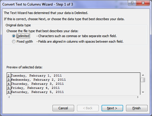3.     Select Delimited and click Next

4.     Select the Coma Delimiter and Space Delimiter. We’re selecting both because our data is separated by comas and spaces. You’ll also notice the ‘Treat consecutive delimiters as one’ box is checked. This just ignores additional spaces in your data so you don’t end up with extra columns.

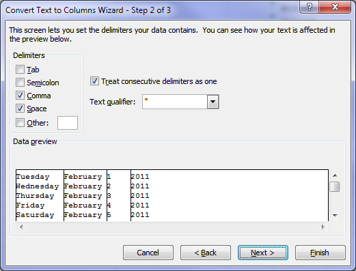You can see in the preview window that Excel has removed the comas and inserted columns.

5.     In step 3 of the Convert Text to Columns Wizard (image below) you can click on each column in the Data Preview and then select the format from the ‘Column data format’ options.

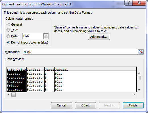We’re selecting to skip the first column, and we’ll leave the other 3 columns as a general format and we’re going to insert the data beginning in cell D2.

Click Finish

Note: Although there is an option to tell Excel that these columns are date formats it isn’t any use to us because each column only has one component of the date, and so Excel doesn’t have enough information to insert the date correctly.

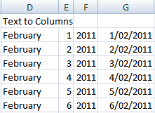
Now our data looks like this, with the original data in column A and the split data in columns D, E and F.

Troubleshooting: If you find your text has come across in a date format it’s because the destination cells were already formatted as a date. You need to format them as ‘General’ before doing Text to Columns.

6.       The last step is to insert a DATE formula that joins our data back together in a date format.

The syntax for the DATE function is:

=DATE(year, month, day)

And our formula is:

=DATE(F2,MONTH(1&D2),E2)

The DATE function tells Excel that the value is a date.

You’ll notice that we’ve had to do a bit of jiggery pokery with the month because it’s text. i.e. the word ‘February’, but Excel needs February represented as the number 2 for the DATE formula to work.

We use the MONTH function to convert the name of the month to a number. The syntax for the MONTH function is:

=MONTH(serial_number)

Our formula is:

=MONTH(1&D2)

Where D2 contains the text ‘February’.

This formula works by telling Excel that there is a date ‘1 February’, which it then converts to the month number ‘2’.

And voila, now we have our date correctly formatted in column G.

Note: before we can go and delete columns D, E and F we need to copy and paste our dates in column G as values. Then we can delete any of the columns we don’t need.

Now, this may seem like a convoluted method, and to a degree it is. But once you get to grips with it you should be able to change a whole column of dates to the correct format in under 1 minute.

Tagged as: text function