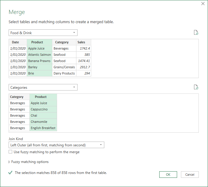
If you've done lookups in Power Query to pull values from one table into another, you may have used a query merge to do this.
Mynda has written previously on how to do an Exact Match in Power Query and an Approximate Match in Power Query
Here I'll be showing you how to use List Functions in Power Query to do both Exact and Approximate matches.
This approach requires a little more M coding but requires less steps and is my preferred method for doing lookups. But hey, I would think that, I'm a coder 🙂
Using List Functions
The key to doing this is remembering that table columns are lists, and as such you can use List Functions to manipulate the data in them.
Watch the Video

Download Sample Excel Workbook
Enter your email address below to download the sample workbook.

Exact Match
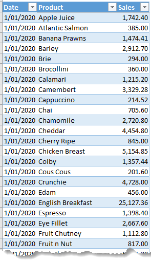
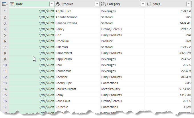
My sample data is a table of sales on different dates for different types of food and drink. This table is named data.
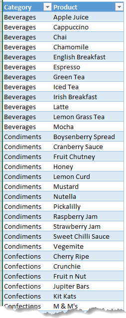
What I want to do is add a column showing the category for each item. These categories are stored in a separate lookup table named categories.
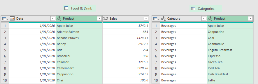
I've loaded both tables into PQ and set categories to load as connection only because I don't need to create a new table from it.
So with both tables loaded into PQ, let's look at what we need to do.
The Food & Drink query needs to get the Category from the Categories table. By looking up the value in the Food & Drink[Product] column in the Categories[Product] column we can get the row number in Categories[Product] that matches.
Using that row number as an index on the Categories[Category] column will return the Category.
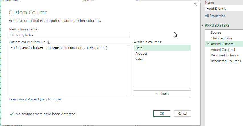
Let's do this step by step. Start by adding a Custom Column and calling it Category Index.
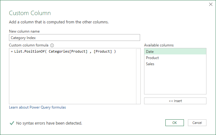
Using the List.PositionOf function, I want to look up in the Categories[Product] column, the value in this [Product] column.
The new column shows the position of each Product in the Categories table.
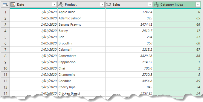
Remember that Lists are indexed from 0, so Apple Juice is in Position 0 of the [Product] column in the Categories table.
Atlantic Salmon is position 65 etc.
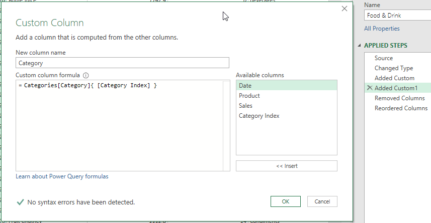
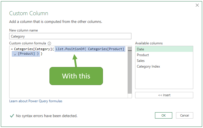
Now that I have this index number I can use it to lookup the category. Create another Custom Column and call it Category.
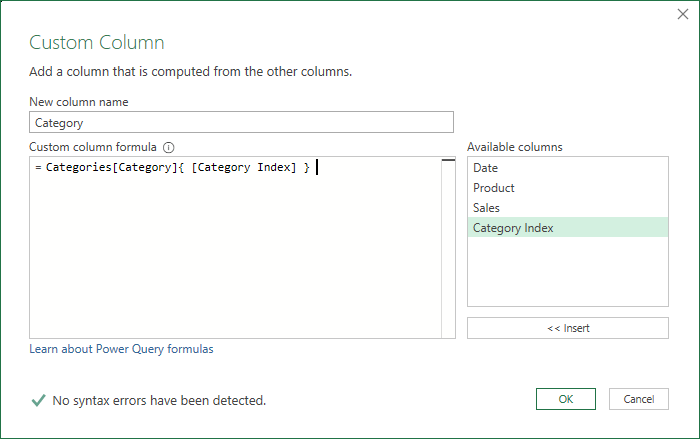
What I need to do here is enter a reference to the value in the Categories[Category] column. This is done by specifying the Category Index value inside curly braces after the Table[Column] reference.
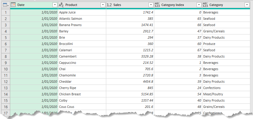
Click OK and this creates the Category column in the Food & Drink table.
Let's do a litle tidying up, We don't need the category Index column now so delete it, and reorder the columns.
Before I finish though, I can make things a little neater. I like reducing my steps and code where possible.
You can see in the Added Custom step that the code creates the Category Index column
And the subsequent Added Custom1 step it uses the values from that Category Index column.
You can take the code List.PositionOf( Categories[Product] , [Product] ) from the Added Custom step, and replace [Category Index] in the Added Custom1 step with it.
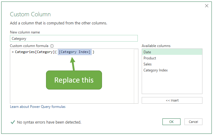
This condenses the code from two steps into one and you end up with the same result.
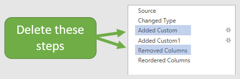
As the Added Custom step is no longer needed, delete it. Also delete the Removed Columns step as all that is doing is deleting the Category Index column. But as the query is no longer creating that column, this step is not needed either. I don't actually need to create the Category Index column at all.
OK so the query is done, load to the sheet and that's our finished table.
Approximate Match
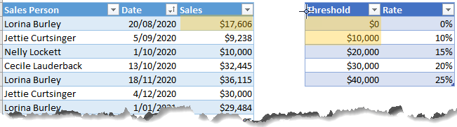
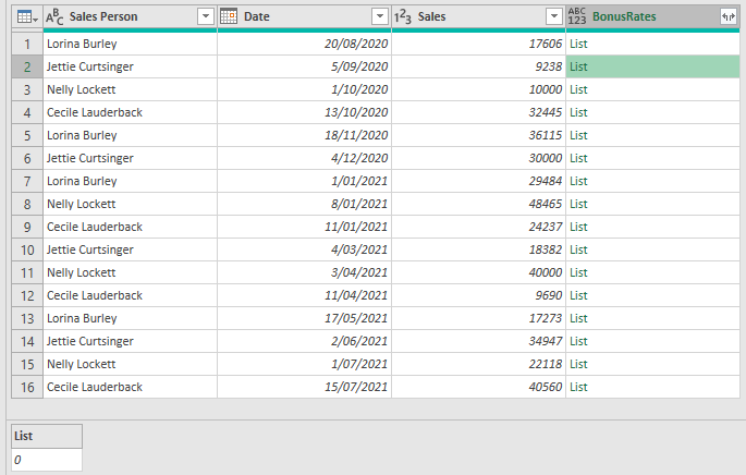
To do an approximate match I'm going to use this table of sales figures for various sales people and add a new column showing the bonus rate they'll get for those sales.
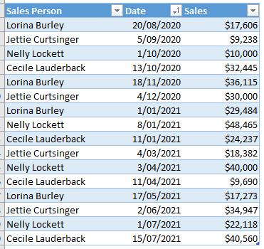
The idea being that you multiply the sales amount by the bonus rate to work out the bonus the sales person gets paid.
The bonus rates are stored in a separate table called excitingly, BonusRates.
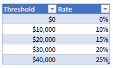
Make sure the table is sorted in ascending order on the Threshold value. It's important to note that the first row has $0 threshold and a rate of 0.
The reason for this will become clear as I explain how the lookup query works
The bonus rate is determined by the sales amount. If you sell $10,000 or more, but less than $20,000 then the rate is 0.1
If you sell $20,000 or more but less than $30,000 then the rate is 0.15, etc
Load both tables in Power Query and set the Bonus Rates lookup table to connection only.
What I need to do here is of course look up the sales amounts in the BonusRates table. But this time I'll use List.Select to create a list of all values in the BonusRates[Threshold] column less than or equal to the Sales Amount
The number of elements in this list will be used as the index to lookup up the bonus rate.
I'll use the first sales value of $17,606 as an example. There are 2 values in the Threshold column less than or equal to $17,606.
The List.Select function creates a list containing 0 and 10000. Then by counting the items in this list, I can use that number to return the 2nd item in the Rate column which is 0.1, or 10%
Let's look at the code. Open the Power Query editor and add a Custom Column called BonusRates and add this code
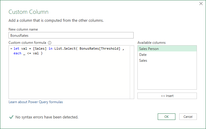
I'll explain what's going on here
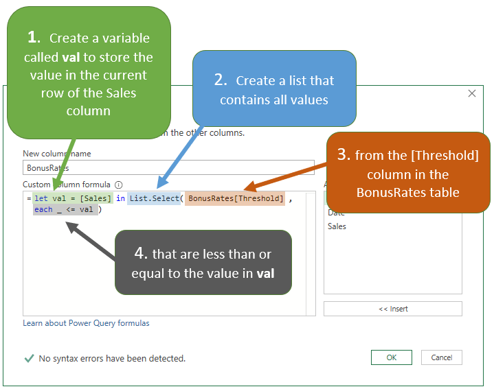
The variable val contains the Sales value in the current row of this table. Remember that the code written here is run for every row in the Sales column.
List.Select creates a list containing all values in the BonusRates[Threshold] column, that are greater than or equal to the value in val.
The each _ is shorthand for the current item in the BonusRates[Threshold] column. It's saying compare val with each item in the BonusRates[Threshold] column
The result of this code is a column of lists.
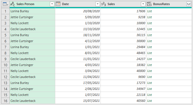
By clicking into a cell beside one of the lists, I can check what is in that list.
For the Sales value 9238 the BonusRates list contains just a 0, because the minimum sale amount to get a bonus is $10,000.
If there wasn't a row in the lookup table with 0 threshold then the list for any sales value less than 10000 would be empty. When the query tried to lookup an index using an empty list it would generate an error. Having the 0 Threshold row means that the code will always create a non-empty list and avoid such errors.
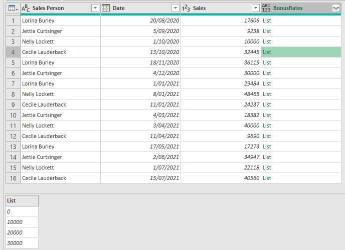
Checking the list in row 4 for the Sales value 32455 shows that the list contains 4 items, because this sale amount crosses the $30,000 threshold.
With this new column of lists I can now count the items in each list and lookup the bonus rate for the Sales amounts.
Add another custom column, call it Bonus Rate, with this code

What we need to do is lookup the value from the Rate column in the BonusRates table, and the number of items in the list created in the previous step is the index to that value.
Remember that lists are indexed from 0 so if list has 2 items then the 2nd item is at position 1. Therefore we have to subtract 1 from the count of items in the list
That's all I need so clicking OK and the new Bonus Rate column is created. I don't need the column containing the lists of bonus rates so I delete that leaving me with this final table.
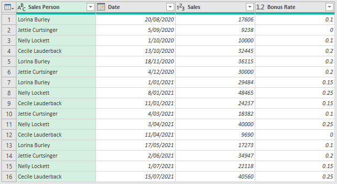
I can now calculate the bonus amount in Power Query, or load this table to Excel and do it there.


I tried to combine the two examples on this page and came up with the following.
This actually retrieves the BonusRate correctly even if Bonus Rates table is not sorted.
And it even works without the line with the 0 in that table.
Bonus[Rate]{List.PositionOf(Bonus[Threshold],
List.Max(
let val = [Sales] in List.Select(Bonus[Threshold], each _ <= val),0))}
It's a great tutorial.
I was just looking to do this in one step.
Nice! Thanks for sharing, Ralf.
Hi Phil,
the Exact Match is working fine considering :
– when it doesn’t match (as expected), I have errors that I want the user take a look at
But now I face errors when I want to load the data.
Do you have any recommandations ?
Regards
You can handle the error with ‘try otherwise’ and return a message instead, like “Investigate”.
Hi Phil
That was a great tutorial exploring the list functions. The {Lists} are at the heart of Power Query and thank you for reminding us that the table Columns are indeed lists objects. I am aware of nested let in statement, but I did not know that the let in block works inside the function as you did with the AddColumns().
I have broken down a bit your Code just to make sure I got the hang of the each _ when we have to reference two table objects and explore a bit more the let in block inside the function.
let
Source = “C:\Users\USER\Documents\DataAnalytics\Power Query\Practice\VlooukUpListFunctions”,
ExtractSalesTable = let
FolderContent = Folder.Files(Source),
BinaryToTable = Table.AddColumn(FolderContent, “ConvertToTable”, each Excel.Workbook([Content])),
SelectColumns = Table.SelectColumns(BinaryToTable,{“ConvertToTable”}),
ExpandedTables = Table.ExpandTableColumn(SelectColumns, “ConvertToTable”, {“Name”, “Data”}),
SelectSalesTable = ExpandedTables{[Name=”Sales_Data”]}[Data]
in
SelectSalesTable,
VLookUp = let
MergeDiscountRate = Table.AddColumn(ExtractSalesTable, “ApproximateDiscountRate”,
each let SalesVal= [Sales],
DiscountRateRange = List.Select(LookUpTable[SalesRange], (DiscountRange) =>
DiscountRange<= SalesVal),
RowIndex = List.Count(DiscountRateRange)-1,
DiscountRateMatch = LookUpTable[Rate]{RowIndex}
in
DiscountRateMatch)
// I have renamed the Threshold Field to SalesRange
in
MergeDiscountRate
in
VLookUp
I enjoy playing around with the nested let in statement, not only for the sake of compacting the applied steps but also to hide the gear icon from the applied steps!
Kind regards
Osorio
Great Osorio. When you learn to manipulate lists, records and tables within columns and other structures you can do some really cool things and save a lot of extra steps in the query.
Regards
Phil
Good day! Thank you so much for sharing this.
Regarding “You can take the code List.PositionOf( Categories[Product] , [Product] ) from the Added Custom step, and replace [Category Index] in the Added Custom1 step with it.” when I try to do it, I face the error below:
Expression.Error: The index cannot be negative.
Details:
Value=[List]
Index=-1
Hi Jan,
Hard to debug the issue without seeing your query and data. Can you please start a topic on our forum and attach your file there.
Regards
Phil
I tried to use this approach today, but in writing the formula it didn’t recognize the fields in the lookup file. Both tables were added to Power Query using a connection only. What might I be doing wrong?
Hard to say without seeing the file, Mark. Please post your question on our Excel forum where you can also upload a sample file or screenshots and we can help you further.
Thanks for your quick response. I did figure out the problem. The formula was sensitive to spaces where I didn’t initially include any. Once I added the spaces as reflected in your written instructions it worked.
Great to hear, Mark.
what if i need to use two or matching criteria to return a value using list.positionof? in your above example, lets say date and product would be the matching values from both table and category is the value i want to return.
Please post your question on our Excel forum where you can also upload a sample file and we can help you further.
How do I formulate date in a cell of one workbook to be incorporated as part of different workbook name
VLOOKUP(M$12,’RPT\SHIFT RPT\2024\1 Jan 2024\[1-25-24 Shift Rpt.xlsx]FTE’!$A$24:$B$24,2)
M$12 is 6-7a
K24 is 1-25-24
Up to now, I have been creating the 10 tab report for each new day using find and replace to change the dates and I know there is an easier way to formulate this. Any help you can give is much appreciated!!!
Hi Lou,
You can use INDIRECT for this. Please post your question on our Excel forum where you can also upload a sample file and we can help you further.
Mynda
How would you do the same thing but instead of needing and approximate match, needing a Text to be found in the reference table…
Find the row that contains this “keyword” in a description column and return the value of other columns in that keywords table
So, table 1 has Transaction Date, Description, Amount (as in any Bank Statement)
Table 2 has Keyword, Category, Payee (Would relate a keyword to categories and payees)
Description has a complex text but if it contains “Keyword” I want to assign Category and Payee to that row.
If description contains keyword then return payee and category for that description…
I hope I made myself clear…
Hi Ricardo,
I’d probably use an approach similar to these with some modifications
https://www.myonlinetraininghub.com/create-a-list-of-matching-words-when-searching-text-in-power-query
https://www.myonlinetraininghub.com/searching-for-text-strings-in-power-query
Can you please post a question on or forum and attach some sample data as it’ll be easier to figure out a solution for you.
Regards
Phil
Please guide: In approximate match case, If I want to calculate bonus for each slab separately and then add these slab-wise bonus amounts, which formula will work? E.g. If sales is 25000, bonus needs to be worked out:
A. For 1st Slab 0-10000 = 0 bonus
B. For 2nd Slab 10001-20000 = 10000 X 10% = 1000 bonus
C.For 3rd Slab, Total Sales 25000 – Slab limit 20000 = 5000 (This difference amount only to be given bonus of this slab). So bonus for this slab 5000 X 15% = 750.
So total bonus A + B + C = 0 + 1000 + 750 = 1750
That’s explained in this tutorial: Power Query VLOOKUP approximate match.
How list.PositionOf will work with multiple criteria?
Thanks.
Hi DK,
List.Position of only gives the position of one thing in a list.
If you want to search for the positions of multiple things you can use List.PositionOfAny
Regards
Phil
Tried to look for previous dates…
Expression.Error: We cannot convert the value #date(2022, 1, 1) to type List.
Hi Joe, please post your question on our Excel forum where you can also upload a sample file and we can help you further.
Thank you so march!
Earlier I’m use merging table, but you solution is better!
I’m beginner and some confusion in let in operator, but I found it in doc:
https://docs.microsoft.com/en-us/powerquery-m/m-spec-let
You’re welcome Gayrat, glad this was useful for you.
regards
Phil
Thanks for sharing. I really like this solution instead of merging and expanding tables to get lookup values. Much simpler and straightforward. However, when I applied this to project where the first table had 10,000+ rows and the second table had 1,000+ rows I had to kill Excel after the query didn’t return in twice the time that it took when using Merge/Expand.
Hi,
Try using List.Buffer() on the lists before passing them into the other list functions. If you still have issues please start a topic on our forum and post your file so I can take a look.
Regards
Phil
Hello . Please solve a problem in FiFo method with PowerQuery and put it on YouTube
Thanks a lot
Ingenious the approach for the approx. match…! thx
Unfortunately M-language (also DAX language) solutions makes it rather complex for many users.
Thanks Danny, if you take our Power Query or Power Pivot courses you’ll start to understand M and DAX.
Regards
Phil