Excel GROUPBY and PIVOTBY Functions

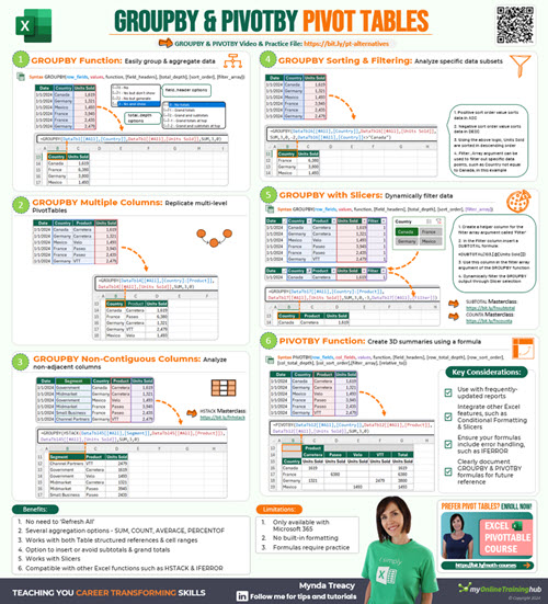
The GROUPBY and PIVOTBY functions are a significant breakthrough in Excel's toolbox of functions.

They let you easily group or aggregate data, a concept that's been around in Excel since the days of PivotTables in 1993 and Power Query since 2010.

But what's exciting about GROUPBY and PIVOTBY is that they simplify this process down to a formula.

This means any changes to the source data are instantly updated in your reports, unlike PivotTables which require a click of the Refresh button to update.

But what about Slicers, which are one of the best features of PivotTables?

Don't worry, I'll share a clever trick so you can still use Slicers with GROUPBY and PIVOTBY.

Note: at the time of writing, GROUPBY and PIVOTBY are only available in Excel for Microsoft 365 Insiders Beta channel. And currently only 50% of Beta users have these functions.

GROUPBY and PIVOTBY Video

Download Excel Workbook & Cheat Sheet

Excel GROUPBY Function Example

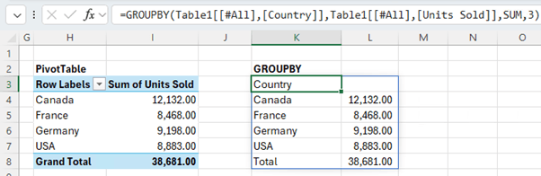
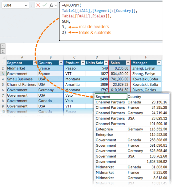
If you're familiar with PivotTables, you can think of the GROUPBY function as a PivotTable that doesn't have any fields going across the columns. In the image below we can see them side by side:

In its simplest form GROUPBY takes the following arguments:

=GROUPBY(

row_fields - Column(s) you want to group by,

values - Column(s) of values you want to aggregate,

function - how you want to aggregate them,

field_headers - include/exclude headers

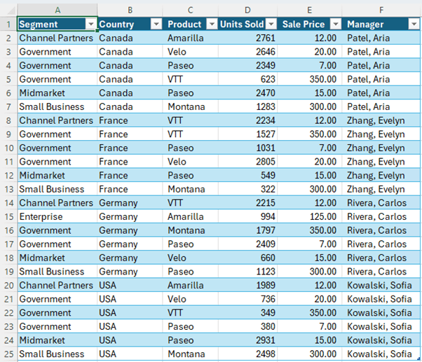
To demonstrate, I'll use this data formatted in an Excel Table called, Table1:

The GROUPBY formula above is referencing the Table using Structured References which makes it relatively easy to read. Here it is again:

=GROUPBY(Table1[[#All],[Country]],Table1[[#All],[Units Sold]],SUM,3)

In English it translates to group the Country column and take the Units sold, sum them and include a header.

See the next section for more on headers.

GROUPBY Function Syntax

The full GROUPBY function syntax is:

=GROUPBY(row_fields, values, function, [field_headers], [total_depth], [sort_order], [filter_array], [field_relationship]1)

Note 1: The 'field_relationship' argument was added after the video above was recorded.

The arguments are explained as follows:

The Row Fields are the columns that contain the values which are used to group rows and generate row headers.

The Values are the columns of data you want to aggregate.

The array or range may contain multiple columns. If so, the output will have multiple row group levels.

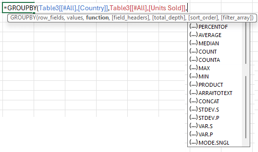
The Function argument is an explicit² or eta reduced lambda (SUM, PERCENTOF, AVERAGE, COUNT, etc) that is used to aggregate values. There's a long list of eta lambdas you can choose from.

Note 2: You can insert your own custom LAMBDA in this argument. See this post for more on how to write custom Excel LAMBDA functions.

A vector of lambdas can also be provided. In which case the output will have multiple aggregations. The orientation of the vector will determine whether they are laid out row- or column-wise. e.g. use HSTACK(SUM,PERCENTOF) to return the sum and percent of calculations across the columns.

Field Headers allows you to specify whether you want to display headers and in what form:

• Omitted: Automatic headers³.
• 0: No
• 1: Yes and don't show
• 2: No but generate
• 3: Yes and show

Note 3: Automatic assumes the data contains headers based on the values argument. If the 1st value is text and the 2nd value is a number, then the data is assumed to have headers. Fields headers are shown if there are multiple row or column group levels.

Total Depth Determines whether the row headers should contain totals. The possible values are:

• Omitted: Automatic: Grand totals and, where possible, subtotals.
• 0: No Totals
• 1: Grand Totals
• 2: Grand and Subtotals
• -1: Grand Totals at Top
• -2: Grand and Subtotals at Top

Note: For subtotals, fields must have at least 2 columns. Numbers greater than 2 are supported provided field has sufficient columns.

Sort Order is a number indicating how rows should be sorted. Numbers correspond with columns in row_fields followed by the columns in values. If the number is negative, the rows are sorted in descending/reverse order.

A vector of numbers can be provided when sorting based on only row_fields.

Filter Array is a column-oriented 1D array of Booleans that indicate whether the corresponding row of data should be considered.

Note: The length of the array must match the length of those provided to row_fields.

field_relationship - specifies the relationship between the fields

• 0: Hierarchy (default)
• 1: Flat

Specify 1 when you have multiple columns to group by and you want to sort by a column other than the first column returned in the formula. Note: when subtotals are included you cannot use 1 for field relationship i.e. a flat table.

PIVOTBY Function

The PIVOTBY function enables you to generate a summarized version of your dataset with a formula.

PIVOTBY is essentially the same as GROUPBY except it has additional arguments for the columns making it adept at organizing data across two axes and performing aggregation on the related values.

Syntax:

=PIVOTBY(row_fields, col_fields, values, function, [field_headers], [row_total_depth], [row_sort_order], [col_total_depth], [col_sort_order], [filter_array], [relative_to]4)

Note 4. The 'relative_to' argument was introduced after the video above was recorded. It's for use with the PERCENTOF function enabling you to specify how the calculation is performed relative to:

• 0 - Column Totals (Default)
• 1 - Row Totals
• 2 - Grand Total
• 3 - Parent Col Total
• 4 - Parent Row Total

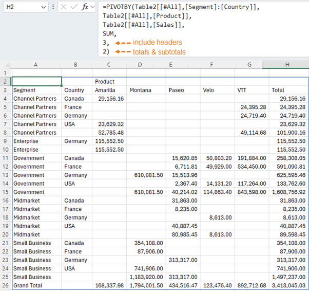
In the example below I've used PIVOTBY to summarise the sales by Segment in the rows, and Products in the columns:

Returning Multiple Columns

You can reference multiple columns in the first argument of PIVOTBY and GROUPBY:

Notice I've used 2 in the Total Depth argument to return totals and subtotals.

Tip: for non-contiguous columns use the HSTACK function to join them e.g. I can join the Segment and Product columns with HSTACK:

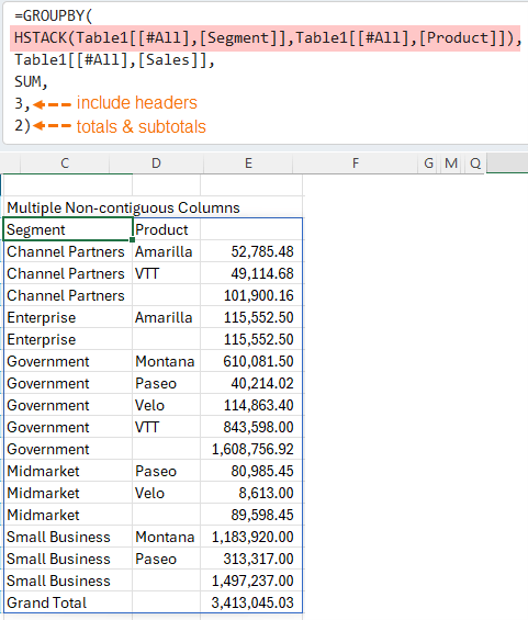
Notice it automatically inserts subtotals at each change in group. We'll look at controlling subtotals soon.

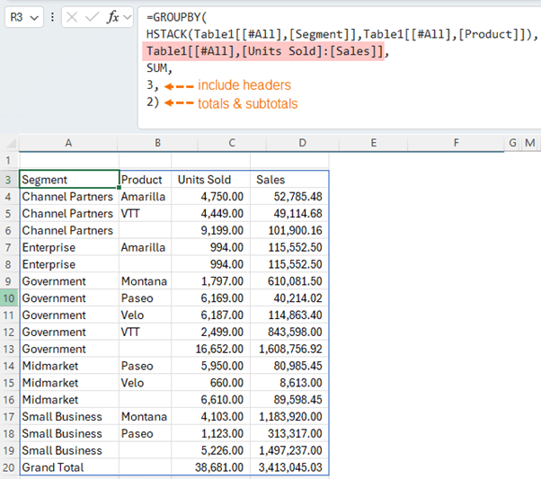
Similarly, we can return multiple contiguous value fields as shown below (for non-contiguous fields use HSTACK):

Tip: you can also rearrange the order of the columns with HSTACK.

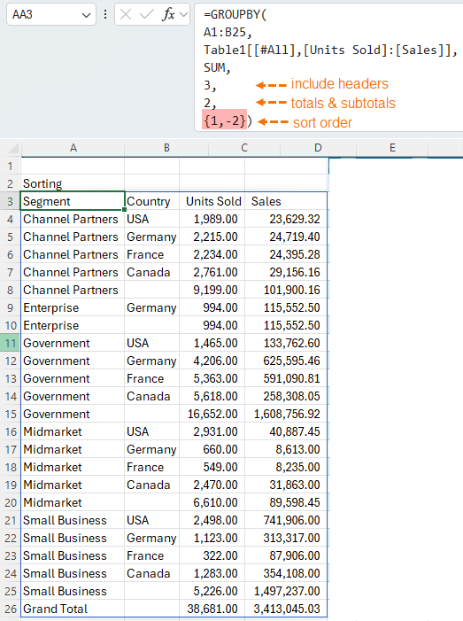
Sorting

The Sort Order argument is a number indicating how rows should be sorted. Numbers correspond with columns in row_fields followed by the columns in values. If the number is negative, the rows are sorted in descending/reverse order.

A vector of numbers can be provided when sorting based on only row_fields.

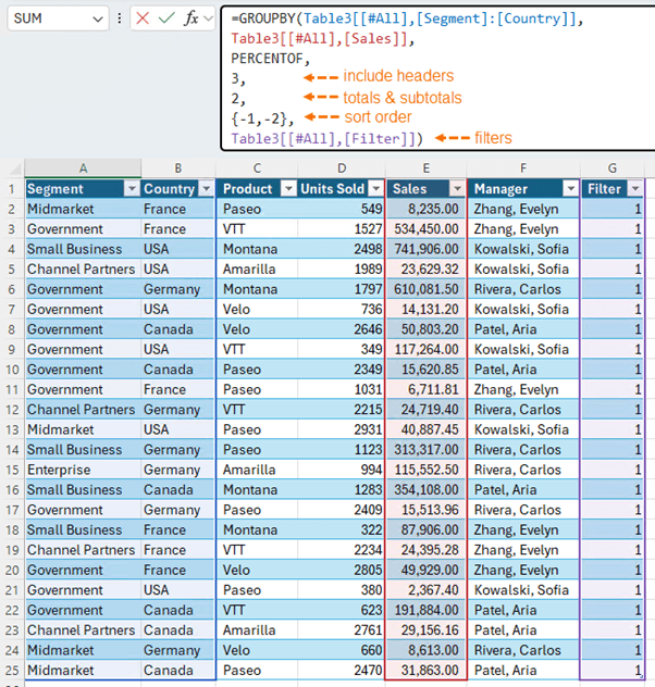
In the example below I've sorted in ascending order by Segment then descending order by Country in GROUPBY, but it works the same in PIVOTBY:

Filtering

The Filter Array argument is a logical test applied to a column that returns TRUE or FALSE Boolean values that indicate whether the corresponding row of data should be included.

Note: The length of the array must match the length of those provided to row_fields. 

In the example below I've filtered the formula to exclude 'Midmarket' from the Segment column.

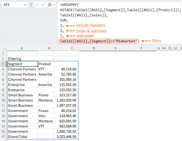
Tip: you can filter on columns not included in the GROUPBY formula result e.g. I could filter based on Country in the above formula.

Connecting GROUPBY & PIVOTBY to Slicers

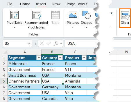
Slicers are one of the best things about PivotTables, so it'd be a shame not to be able to use them with these new functions. Thankfully, we can use Slicers with Excel tables and leverage the filter argument to pass the filtered state to the GROUPBY and PIVOTBY functions.

First, select a cell in the Table and add the Slicers you need via the Insert tab > Slicers:

Then add a column to your Table to detect if the row is filtered or visible using the SUBTOTAL function or AGGREGATE function. These functions can include or exclude rows hidden by a filter.

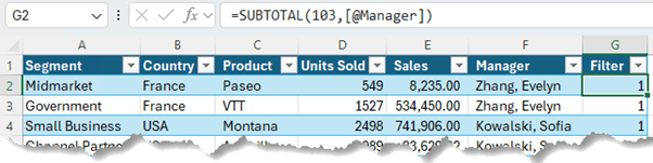
103 in SUBTOTAL is the COUNTA function that ignores hidden/filtered values. If the row is visible, SUBTOTAL returns 1, which is equivalent to TRUE and if it's hidden it returns 0 which is equivalent to FALSE.

Tip: the formula can reference any cell in the row that will never be empty.

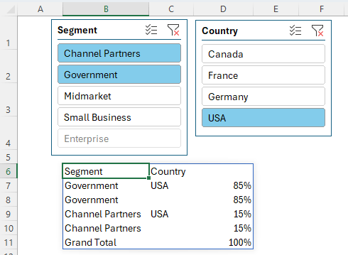
Then simply reference the Filter column in the Filter argument of GROUPBY or PIVOTBY. Visible rows = 1 and are included in the GROUPBY formula:

Now when you make selections in the Slicers, the GROUPBY or PIVOTBY formulas will filter accordingly:

Automatically Format Total Rows

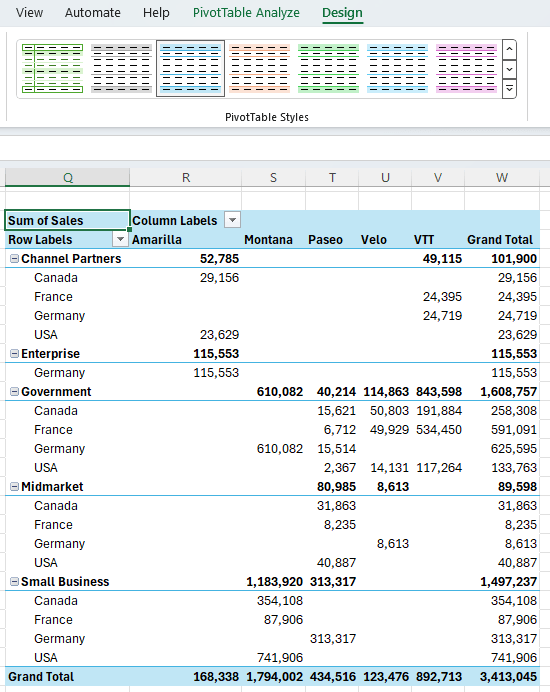
Another nice feature of PivotTables is their built-in formatting that automatically highlights totals and subtotals:

With GROUPBY and PIVOTBY we can use Conditional Formatting to replicate this and have it dynamically update with the results of the formula:

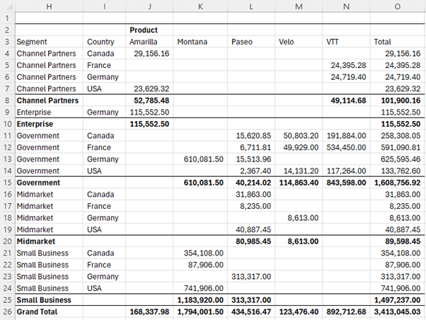
We can rely on the second column having a blank cell on the subtotal and total rows. All we need to do is detect if the cell is blank and if so, format the row in bold font and a cell border.

To set up a conditional format, go to the Home tab > Conditional Formatting > New Rule > Use a formula to determine which cells to format.

In the 'Format values where this formula is true' field, select the first cell in the second column and set the absolute reference to the column only and check if that cell is blank:

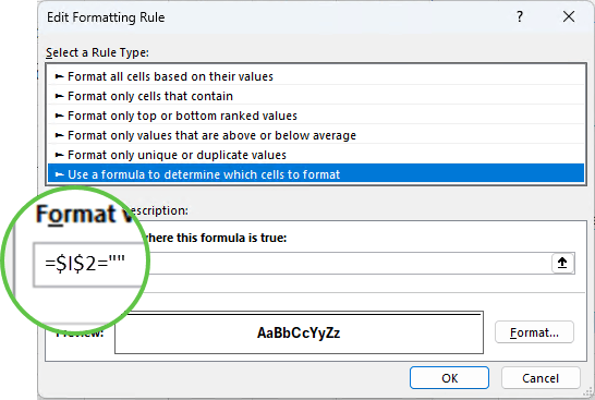
Note: you can't use ISBLANK here because technically the cell isn't blank because it contains a formula.

Then go to the Format tab and format the font bold and on the Border tab add a border to the top of the cell:

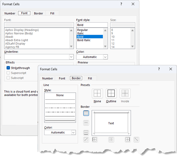
Tip: you could create another rule and add fill colour to the Grand Total to replicate PivotTables.

PivotTable Advantages

There is no doubt that these two functions are game changers for grouping and pivoting data in Excel, but there are some good reasons to still use PivotTables:

• Working with Big Data: PivotTables don't require you to bring the data into the grid to summarise it. PivotTables can reference data in queries or external files enabling them to work with a lot of data with a relatively small impact on the file size. GROUPBY and PIVOTBY require the data in the grid.
• Multiple Aggregations: if you want to add multiple aggregation types e.g. see the data summed, averaged, and counted it's super easy in a PivotTable, whereas writing this into a GROUPBY or PIVOTBY is complicated.
• Backward Compatibility: All versions of Excel support PivotTables. Whereas GROUPBY and PIVOTBY are only available to Excel users with Microsoft 365.

For these reasons, PivotTables will still be an important tool in your Excel skillset. Master PivotTables in my PivotTable Quick Start course.