Excel Pivot Tables are one of the most powerful tools at our disposal, and once you understand how they work, they’re actually quite easy to insert and modify.
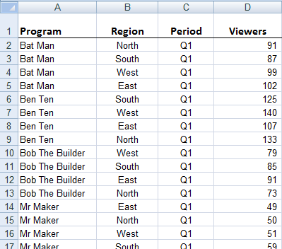
In this example we’re going to work with a small amount of data (see image below) for illustration purposes, but Pivot Tables are in their element with huge amounts of data laid out in a tabular format.
Forget Filters and Subtotal, Excel Pivot Tables can do both of these and more in a few seconds.
Watch the Video

Download Example Workbook & Cheat Sheet
Enter your email address below to download the workbook and cheat sheet.

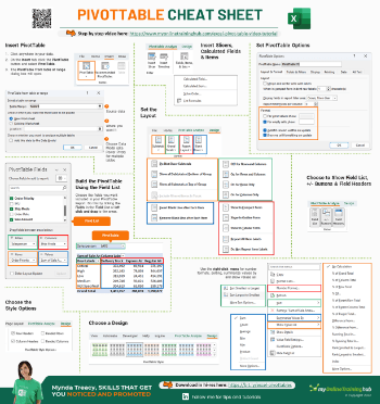
- Download the Cheat Sheet.
- Download the workbook and practice as you go. Note: This is a .xlsx file. Please ensure your browser doesn't change the file extension on download.
Getting Started with Excel PivotTables
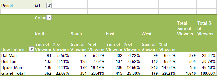
Taking the data below, let's say we wanted to SUM the number of viewers by program going down the rows, then by Region going across the columns and only show Q1 (you can't see it here but there is data in the table below for Q1 through to Q4).
The easiest solution is to insert a Pivot Table like this:
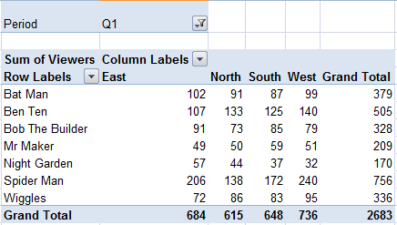
Note: In the above example we summed the viewers, but instead of, or in addition to SUM, we can COUNT, AVERAGE, PRODUCT and more. I'll cover how to do that in a moment.
We can also change the formatting and customise the default ‘Row Labels’, ‘Column Labels’ and ‘Sum of Viewer’ headings to make the report more polished. We'll get to that soon.
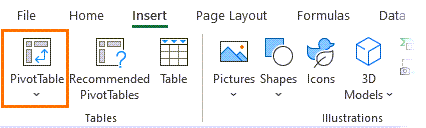
How to Insert Excel Pivot Tables
- Click anywhere in your data
- On the ‘Insert’ tab click the ‘PivotTable’ button and select ‘PivotTable’.
- The Create PivotTable dialog box will open.
- I’ve chosen to insert mine in cell F2 on the sheet where my data is for this tutorial. Below is how your worksheet will look after step 3. In the right hand section of your screen the Pivot Table Field List window will open and a place holder will be entered beginning in the cell you’ve chose in the previous step, in my case F2:H19.
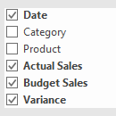
- The first thing you need to do is choose the fields you want included in your Pivot Table Report. We do this in the Field List window.
- To insert the Pivot Table shown in the above example, and below, my Field List looks like this:
- First you have to add another Value field by dragging, in our case, ‘Viewers’ from the ‘Choose fields to add to report’ section down to the ‘Values’ area. You’ll notice that Excel will put a Values field in the ‘Column Labels’ area as well as the Values areas. This is because it’s performing the calculation for each column of data. You can change it to calculate for each row by dragging it to the ‘Row Labels’ area.
- Open the ‘Value Field Settings’ dialog box (click the down arrow and select it from the list) and select the ‘Show values as’ tab.
- From the drop down list you can choose the type of calculation you want.
- Give your calculation a custom name before clicking OK.
- No blank rows or columns.
- Each column must have a heading. This heading will be carried over to label your Pivot Table rows and columns.
- Make sure your source data is formatted correctly. That is if they're dates, format them as dates and so on.
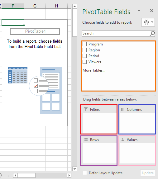
- If the Field List disappears click anywhere on the Pivot Table and it will reappear. If it still doesn't appear, right click the PivotTable > Show Field List.
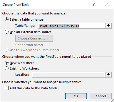
a. Excel will automatically select the range of data, but you can change this here if you need to by modifying the range in the Table/Range field. You can even choose an external source but for most people using your own data will be all you want, so we’re not going to cover that here.
b. Tell Excel if you want your Pivot Table in a New Worksheet or in the Existing Worksheet. If you choose Existing Worksheet you will need to tell Excel the top left cell that you would like your Pivot Table to begin in. If you choose New Worksheet Excel will insert a new worksheet in your file and insert it there.
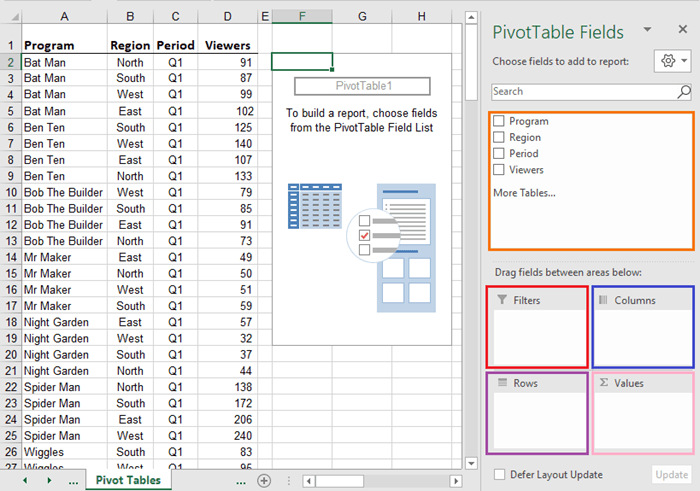
a. By ticking the Fields from the list you can tell Excel which fields you want in your report.
b. By default it will add any labels to the ‘Row Labels’ area, and any columns it detects as values will go into the 'Values' area. To move them, simply drag and drop the fields to the area you want.
c. If you’re inserting your Pivot Table on the existing sheet you will see it take shape as you make your selections in the Field List.
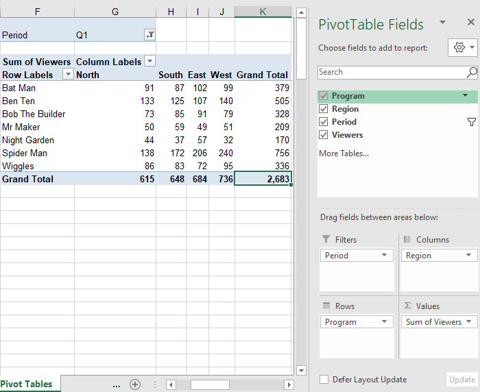
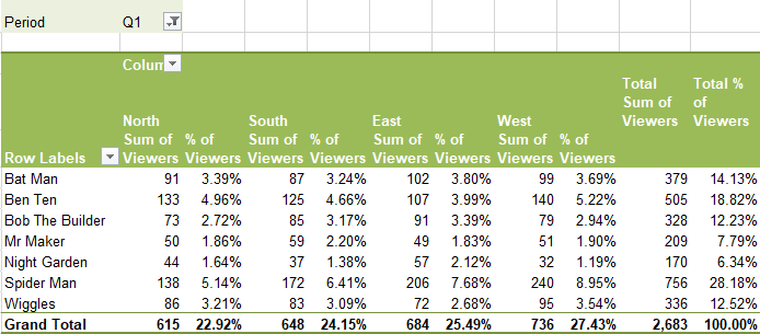
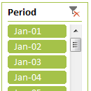
You can see I’ve set the Period Q1 (cell G1) as a ‘Report Filter’, the programs are my Row Labels, the Regions are my column labels and the Sum of Viewers are my Values.
Ok, now let’s look at how we can customise it.
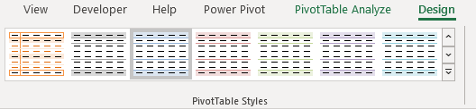
Excel Pivot Table Styles
In Styles enable you to make your Pivot Table cool with very little effort.
You’ll notice you now have two new tabs in your Ribbon. Go to the Design tab and here you can choose from a huge range of predefined styles. You can even save your own in keeping with your corporate image.
Just look at how much more professional mine looks with a few clicks of the mouse.
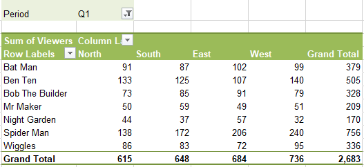
I've also changed my ‘Row Labels’ and ‘Column Labels’ headings by typing new names directly into the cell.
Preserve Pivot Table Formatting
You can also format your Pivot Table Report manually using the Fonts etc. on the Home tab of the Ribbon, plus you can resize columns and rows.
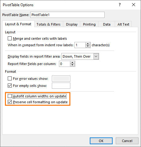
If you do this there are a few preferences you should set so that your formats aren’t lost on refresh.
Right click anywhere on the Pivot Table. Select ‘PivotTable Options'. The following dialog box will open. Make sure you tick the ‘Preserve cell formatting on update’ preference and ‘Autofit column widths on update’ is NOT ticked.
Change Default Pivot Table Value Calculation
Remember at the beginning I said in the Values you aren't limted to just SUM. You can also COUNT, AVERAGE, PRODUCT and a few more.
By clicking on the down arrows beside the Report Filter, Column Labels, Row Labels or Values areas you can access tools that will allow you to modify the settings. This is also where you can change whether the Values are SUM of, COUNT of, AVERAGE of and so on.
To change the VALUES from the default, select ‘Value Field Settings’ from the list by clicking the down arrow beside, in our case, Sum of Viewers.
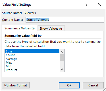
The ‘Value Field Settings’ dialog box will open and you can choose a different calculation from the list on the ‘Summarize by’ tab as shown below.
You can also give the field a custom name.
Note: you can have more than one value in your Pivot Table. For example, you might want to SUM and COUNT the values. Simply drag the field you want from the 'Choose Fields to add to report' list in the Pivot Table Field List into the Values area and alter the Value Field Settings as listed above. (See the next section for instructions on how to add another value with screen shots.)
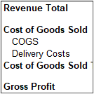
Insert a Predefined Pivot Table Calculated Field
Excel has a list of predefined calculations you can select from. Note: You can also insert a custom calculated field, but we’re not going to cover that here as I think these are better added to your source data and brought into your Pivot Table as a field. It’s less prone to error with this approach.
To insert a calculated field from the predefined list available:
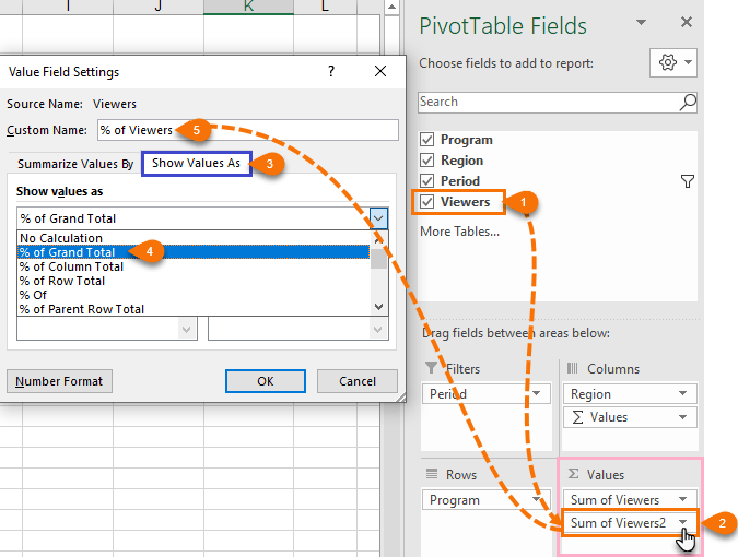
In my example below I inserted a '% of total' field and gave it the custom name ‘% of Viewers’.
Pivot Table Filters
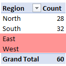
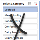
What say we wanted to only show data for a few of our programs? We can filter our row labels by clicking on the down arrow beside ‘Row Labels’. And just like regular filters we can instruct Excel to only display the values we choose.
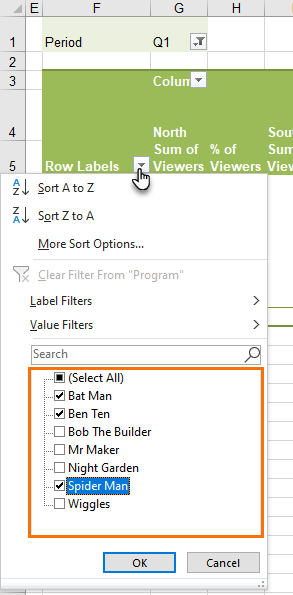
Note: in this filter we can also sort our row labels.
Filters can also be applied to column labels.
Changing the Pivot Table Orientation
You can have more than one field in each area. For example, what if we wanted to see the data grouped by region down the rows? It would look like this:
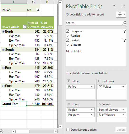
Simply rearrange the fields in the Field List by dragging and dropping the fields to the area you want.
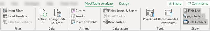
Pivot Table Tools
You will also notice you now have two new tabs in the Ribbon for Pivot Table Tools; Analyze and Design.
Source Data Rules for Excel Pivot Tables
If your data is not in the correct tabular layout for PivotTables, check out the video below on how to easily fix it with Power Query:
Want More
Get up to speed with PivotTables fast in our PivotTable Quick Start course.
And why not visit our list of Excel formula examples. You'll find a huge range of topics including formulas (all explained in plain English), plus more on PivotTables and other Excel tools and tricks. Enjoy 🙂


 Excel Named Ranges Explained

Scott V
Is there a way to color code the slicer buttons?
Mynda Treacy
Hi Scott,
Yes, you can create a custom Slicer style.
Mynda
kevin
I have a dynamic array in A2.
Why will this work in column C =CHOOSECOLS(A2#,2)/SUM(CHOOSECOLS(A2#,2))
but this will not: =LET(cc2,CHOOSECOLS(A2#,2),cc2/sum(cc2))
Mynda Treacy
Hi Kevin,
You cannot use a name that is also a cell reference i.e. CC2. Change CC2 to something else, e.g. ary
Mynda
Ayodeji Tobi
What is the importance of this pivotal table.
Mynda Treacy
PivotTables are an easy and efficient way to summarise and analyse data. They’re an important Excel skill to have.
Lubenica
How to consolidate in one pivot more different sheets?
Tnx
Mynda Treacy
Hi Lubenica, you need to use Power Pivot if you want to create PivotTable reports using data from multiple sheets.
Sal
Hi Mynda,
Column C is players SCGA index (not needed in the query), column D is players handicap. I am trying to get all the header names in the first row then move the first row to headers. My understanding of the format is that there should be 18 rows for each player. My stumbling block is getting 18 holes in a column and also the 18 pars in a column. I’m getting 18 holes plus 18 pars then repetitive groups of pars all in in one column. The par column is 18 blanks then 18 pars then repetitive pars in one column. I can’t seem to get just the information needed in each of these columns without losing necessary data. Advise?
Mynda Treacy
Hi Sal,
Please post your question and Excel file on our forum so I can provide an Excel file in return.
Thanks,
Mynda
Sal Veltri
I have data that is given in the form of a report. I am trying to make a pivot table to do some additional data manipulations. I have been working on this for five days with no luck. This is a link to my data and the work I’ve been able to accomplish, any help would be greatly appreciated.
Mynda Treacy
Hi Sal,
You’re on the right track with your query, but I don’t know what columns C and D represent, presumably one is the player’s handicap, but I’m not sure.
Please post your question on our Excel forum where you can upload your file after you add headings to the columns that are missing information. Then we can help you further.
Thanks,
Mynda
salim
Dear Mynda
kindly send me advice financial formulas in excel
Mynda Treacy
Hi Salim,
Here is a list of our function tutorials: https://www.myonlinetraininghub.com/excel-functions
Mynda
Salim Gul
dear Mynda
kindly guide me how to put the financial formula
=IFERROR(IF(Loan_Not_Paid*Values_Entered,Principal,””), “”)
Loan amount $5,000.00
Annual interest rate 5.50%
Loan period in years 5
Start date of loan 24-12-18
Monthly payment $95.51
Number of payments 60
Total interest $730.35
Total cost of loan $5,730.35
No. “Payment
Date” “Beginning
Balance” Payment Principal Interest “Ending
Balance”
1 24-01-19 $5,000.00 $95.51 $72.59 $22.92 $4,927.41
2 24-02-19 $4,927.41 $95.51 $72.92 $22.58 $4,854.49
3 24-03-19 $4,854.49 $95.51 $73.26 $22.25 $4,781.23
4 24-04-19 $4,781.23 $95.51 $73.59 $21.91 $4,707.64
5 24-05-19 $4,707.64 $95.51 $73.93 $21.58 $4,633.71
6 24-06-19 $4,633.71 $95.51 $74.27 $21.24 $4,559.44
7 24-07-19 $4,559.44 $95.51 $74.61 $20.90 $4,484.84
8 24-08-19 $4,484.84 $95.51 $74.95 $20.56 $4,409.89
9 24-09-19 $4,409.89 $95.51 $75.29 $20.21 $4,334.59
by self i hope you undarstand what i am want to learn
Mynda Treacy
Hi Salim,
Please post your question on our Excel forum where you can upload a sample Excel file, which will help us understand what you’re trying to do.
Mynda
salim gul
dear mynda
thanks for reply
(100-98)/(98*50/150)
i want to above equation in advace way to such as sumif, sumifs etc which ways you have explained please guide me how i set formula
Mynda Treacy
Hi Salim,
No problem, please post your question and a sample Excel file in our forum so we can see your question in context. I can’t explain it based on your example above.
Thanks,
Mynda
salim gul
(100-98)/(98*50/150)
kindly guide me how i set formula in excel pivot. above equation
Mynda Treacy
Hi Salim,
You wouldn’t put a formula like this in a PivotTable, normally PivotTable formulas refer to the field in the PivotTable.
Mynda
Gehan
This is a great explanation for Creating a PivotTables. I use it in my work but I didin’t understand it. I am just using it as I learnt from my colleagues. But now I understand how to use it probably and make any changes I want to make it looks better.
Thanks a lot
Ge
Mynda Treacy
Great to know we could help, Gehan 🙂
Philip Treacy
You’re welcome, glad you found it useful.
GHT
Hi
This was the first time i really understood what pivot tables are because i always don’t have the mood to spend much time on learning, but your training are very fast and easy to learn and was very useful to me.
Thanks a lot.
God bless you.
Mynda Treacy
So glad we could help you get started with PivotTables 🙂
Isaac Hamisi M
Very valuable insight. and easy to understand presentation
Mynda Treacy
Glad you found it useful, Isaac.
hicham
Very well explained, thanks a lot!
Mynda Treacy
Glad we could help, Hicham.
Paranam Kid
Here’s a challenge for you: is there a way to have a pivot table column with an average calculation?
Example: I have 20 sales records spread over 4 months. The standard average calculation Excel uses in the pivot table is total sales divided by 20. But I want total sales divided by 4.
I have not been able to find how to do this. Suggestion?
Catalin Bombea
Well, It’s your challenge in fact, we have the answer 🙂
You have to calculate the number of months between the minimum date and the maximum date from the dates column, and divide your sales by the result.
Create 2 defined names:
MaxDate with the formula: =Max(Table1[Date])MinDate with the formula: =Min(Table1[Date])
The following formula will return the number of months between those dates:
=(YEAR(MaxDate)-YEAR(MinDate))*12+MONTH(MaxDate)-MONTH(MinDate)Please let me know if this is what you wanted.
Cheers,
Catalin
Paranam Kid
Thanks for your quick reply Catalin.
I do not need to calculate the number of months between dates, but rather have the average sales values shown in the pivot table. The so-called Value Field Settings offer an Average, but that Average is not what I want.
Is there a way I can have a pivot table column with the Average I want (i.e. total sales divided by number of months)? If I misunderstood your answer please expand.
Catalin Bombea
Hi,
I think it’s best to upload a sample file with your sample data structure, You can prepare a manual sample of the desired result, compared with the default excel pivot table result. I’ll prepare an example based on your file, it’s much easier to understand when you see the example. Please open a new ticket on Help Desk and upload the file there.
Cheers,
Catalin
Paranam Kid
Hi Mynda,
many many thanks for your reply, and so quickly. I appreciate it.
Well, I learned something today about rolling averages in a pivot table.
Looking at it in the context of my file, I have some remarks:
* I don’t really want a rolling average, but simply an average for the current calendar year. The current year is only 4 months, so I want the average for the current 4 months. Next month I want the average for 5 months, and when the pivot table refreshes I want the average to be updated automatically without any interference from me
* having a column for calculated fields by position requires a certain amount of maintenance, as you point out in the tutorial, whether the column is at the end of the columns of months or at the beginning. To me the monthly maintenance means the solution is more of a workaround, therefore somewhat unnatural. Maybe this conclusion is wrong, but that’s the feeling I get.
So, after studying your solution & thinking about my observations & wishes I came up with is the following.
* I put an independent column to the left of the pivot table. That way the column is not “overrun” as the pivot table expands every month
* in a cell at the top I have put a COUNTA formula, which counts the number of cells that have text in them, in this case name of month. The range to count is 12 columns.
* in the cells below that I have put a formula dividing the sum of 12 contiguous cells (of which currently only 4 are filled for each row) divided by the number of months as counted above.
Although not part of the pivot table, this way I have an up-to-date average till the end of the year. Then next year I will insert a new column for 2017. However, I do see possibilities in some of my other files for rolling averages in a pivot table.
Once again, thanks a lot for your help & pointing out the rolling average possibilities & the position calculations.
Best regards,
PK
Mynda Treacy
That’s the great thing about Excel; there’s always a solution, you just need to know exactly what you want and you’ll find a way 🙂 I’m glad you found something workable for you.
Something for you to consider is Power Pivot, which has the capability to do time intelligence custom columns/items known as measures that are way beyond what’s possible with regular PivotTables.
Mynda
Luis nBarraga
Hi Mynda!
In your article “Pivot tables explained” I tried the link to download the workbook, but only a lot of giberish returns, no excel book. Please send a repaired link.
Thank you!
Catalin Bombea
Hi Luis,
Try to right click-Save Target As…, it should work.
Catalin
Peter
I use Excel mostly privately now & have been getting more & more interested in it, in good part thanks to this amazing site. The language is clear, the examples are really useful, in fact Mynda has the ability to make Excel look easy & fun. Are you sure she was not a teacher in a previous life, rather than an accountant? Just kidding.
I keep track of my daily expenses & had set up a sheet for it. But 1 of your pieces of advice is to use a tabular table with 1 record per row, so I am currently converting my data to a Table, using that amazing reverse table tool you recommend elsewhere.
So now I have a table with 3 columns: date (yyyy-mm-dd), expense item (15 different items or categories), value. On the basis of this I can make a pivot table. The PT gives totals (and/or averages and/or ….) per item and a Grand Total.
But I would like to have totals per item per month (in a horizontal direction), and eventually per year. I believe there is a simple way of doing this, but I have not been able to figure it out. Can you put me on the right track please?
Thanks in advance for your help.
Mynda Treacy
Hi Peter,
Great to know you’re finding our tutorials useful and easy to follow.
Now that your data is in the perfect format you can use the PivotTable group tool to group your dates.
Tip: Drag the dates into the rows area and group from there. Then you can move them to the columns area if you prefer.
Please let me know if you get stuck.
Kind regards,
Mynda
Peter
Yes, that worked, Mynda. Thanks a lot :-))
DEEN
please instruct how spell number to word currency.
there is any other way than macro?
thanks.
Philip Treacy
Hi Deen,
You have to use a macro to do this. I’ve written a blog post on it https://www.myonlinetraininghub.com/convert-numbers-currency-to-words-with-excel-vba
Regards
Phil
Wesley Vanitou
Hello,
First of all your site in really amazing i can believe how much infos you share. I write you because i have an issue with adding a comment colunm before my pivot table data. When I try to filtering the comment doesn’t match anymore the comment i made. Is there a way to fix that ?
Thanks a lot for the time you’ll take to read this.
Have a nice day.
Catalin Bombea
Hi Wesley,
Please upload a sample file to our Help Desk, with detailed description of the problem, it’s hard to say without seeing the problem, i will gladly help you.
Cheers,
Catalin
JO Tan
Dear Sir,
I’m always received your e-mail of “his week’s Excel Newsletter.”
I’m not good in excel and slow learner, but I’m interest and happy to receive it,
at least I can know HOW powerful of excel can be work!
It is very useful to have free “Download the Excel Workbook” for us to learn and can have some excerise with it .cause sometime after reading your explantion of excel work , may confuse and not sure, after download the excel workbook, it help me alot (I’m not good in English Language).
Really amazing and thank to always share with it to have free Training to me.
Thank you very much
Yours Sincerely,
JO Tan
Singapore
Mynda Treacy
You’re welcome, Jo. 🙂
Thank you for taking the time to leave your feedback.
Mynda
samson yanga
highly appreciate that, the system is good
Marti
Huge thanks for this blog. It is the best Excel tutorial resource so far. Well written, easy to follow and the workbook is just priceless! Thank you again!
Mynda Treacy
Aw, thanks Marti 🙂 Great to know you’re finding it useful.
Mynda
dav
Can you please provide working questions to this exercise? For example, instead of you saying, “put this value in this field,” can you say, ” group the number of viewers per region.” Thats just an example.
In that way, people will learn much better than if just given instructions that dont make sense to them.
Mynda Treacy
That’s a great idea, Dav.
Thanks,
Mynda
dav
If you dont mind could you post just a few questions for this exercise? Just for under the headings:
1) “Insert a Predefined Calculated Field”.
2) “Change Default Value Calculation”.
3) “Changing the Orientation”.
It would help me learn better. Thanks.
Mynda Treacy
Hi Dav,
I’d love to but I don’t have time right now to create some custom Q&A for you, sorry.
I’m sure if you download the file and replicate the steps above you’ll see it’s quite straight forward. You can’t really ‘break’ a PivotTable so have a play around with it and experiment.
Mynda
Sagar Kandhare
Hi Mynda,
I think it’s easiest method to learn Pivot Table.
Thank you.
Regards,
Sagar
Mynda Treacy
You’re welcome, Sagar 🙂
Laura
I have a strange thing happening in my pivot table. When I create a pivot table it’s perfect with nothing strange. I hit refresh and it randomly picks a cell and puts a box around it. The box is checked in PivotTable Options to Preserve cell formatting on update, so I don’t know why it’s doing it. If I remove the box and save and then go in and uncheck the box in options to keep the settings and hit “ok” and then go back into options again and recheck the settings and hit “ok”. Now when I hit refresh it’s fine. Any idea as to why it’s happening at all? Nowhere in the original spreadsheet are there any lines. And it doesn’t happen on other sheets within the same workbook. Any ideas?
Mynda Treacy
Hi Laura,
That does sound strange. I’d need to see the workbook and mischievous PivotTable to be able to tell what the problem is. Are you able to send it to me via the help desk?
Kind regards,
Mynda
Elizabeth Avila
Great presentation and very easy to follow, which is very important in learning.
Mynda Treacy
Thanks, Elizabeth. Glad you found it useful 🙂
MARTIN THOMAS
Respected Madam
how to create pivot table using flat data table
Thanking you
Martin thomas
Mynda Treacy
Hi Martin,
You can create a PivotTable with a flat data table just as you would with a tabular data table. I does have some limitations though, which I explain here under the heading ‘Flat Data Table’.
Kind regards,
Mynda
Robin
This website is really a great addition to online free sources of learning excel, I hope it has more and more contents.
Mynda Treacy
Thanks, Robin.
Maria Schneider
Hello,
I am not so new to Pivot tables, but I always love to read all your posts … there is always something new I never tried.
But I did not find anything on “showing text in pivot tables”. Is there a way to force the pivot table to show “text”, not calculate something?
Or am I trying to do something which I could achieve much easier with another excel function?
Example:
I have projects sorted in a table:
Project Project Leader 1 Project Leader 2
ProjectA Justin Thomas
ProjectB Justin Philippe
ProjectC Mynda Philippe
ProjectD Justin Thomas
What I would like to have is like a cross table of the project leader combinations:
Justin Thomas Philippe
Justin Project A Project B
Project D
Mynda ProjectC
The only thing I know for sure is the possible combinations of project leaders.
Maybe you have an idea?
Thank you very much!
Maria
Catalin Bombea
Hi Maria,
Showing text in data fields is not possible in a pivot table, only in header row or column.
For that cross table, to create a formula to combine project leaders you have to provide the combinations algorithm , if you can upload a sample table with your data and details, i will try to help you to find a solution.
You can use our Help Desk to open a new ticket for support.
Catalin
gopiraj
it very useful
Mynda Treacy
Thank you, Gopiraj 🙂
Manish
I use pivots extensively to aggregate data at certain levels. Anyways, the input file that I use to create multiple pivots has undergone constant change i.e. column aa through ac are now added and original columns displaced, old columns deleted, and so forth.
Everytime a new column is added within the named_range of Pivot data — the pivot takes in the new column without being intelligent about the header that defines it, meaning it just takes whatever column now replaced the original column even if the orignal column is now next column — which has caused a lot of headache on my side, as I have formulas that are based on these columns. Questions – a) Is this how pivots work or there is something wrong that I am doign while refreshing pivots, and b) is there a smarter way to define formulas so that atleast they capture data from the right column (column with specific header)?
I’d appreciate if someone could shed more light here.
– Manish
Mynda Treacy
Hi Manish,
That sounds normal to me. The PivotTable just pulls in the data you give it, it cannot tell if the name of a column has moved/been renamed.
I recommend you use the GETPIVOTDATA function
Kind regards,
Mynda.
Robert Singh
Dear Mynda,
Thanks for your wonderful comments for every separate problem. Its really helpful.
Could you assist me to develop a reporting template from where I can generate other reports?
For an example:
Children A (girl) ID: 2002 participated 4 programs in FY 2014
Children B (Boy) ID: 200 participated 8 programs in FY 2014
Children C (girl) ID: 302 participated 3 programs in FY 2014
Children D (girl) ID: 402 participated 6 programs in FY 2014
The programs are as follows: (Health, Education, Sponsorship, Economic, Nutrition, WASH, Rights, Against Violence etc)
Please be noted that there are more than 4000 children involved in different projects. How can I get all the related information at a glance ending the year. How the data import system would be develop?
It would be so kind of you if you kindly assist me out.
Thank you in advance for your kindness.
Robert
Catalin Bombea
Hi Robert,
Can you upload a sample of your workbook, to see your data structure? What do you mean by “data import system” ? You want to import data from an external source? If so, please give me more details on what you are trying to do, i will gladly help you.
You can use our Help Desk:
Cheers,
Catalin
abdullah
Thanks for the Pivot table tutorials.
They are an amazing tool with power to filter out and summarize.
it was a situation in a project where nothing except manually filtering would take hours.
I dont know how i would have done without pivot tables. In my situation i used pivot table twice on the same data which gave me summaries which was amazing.
Thanks again for such a wonderful site and the tips.
Mynda Treacy
🙂 You’re welcome, Abdullah. I am a big fan of PivotTables too.
Kamran
Please be guided,
Insert a Predefined Calculated Field – Step 3
Drop Down List dosn’t have “% of Total”
Catalin Bombea
Hi Kamran,
Can you please be more specific? Predefined Calculated Fields are available for Values field, not for Row/Column Label, or Report Filter, maybe this was the problem;
Also, it’s very useful to know the version of excel you are using; a sample of your workbook would be great help for us to understand the problem, you can upload it via Help Desk
Cheers,
Catalin
Raza
@ Mynda,
Thanks for the reply and I re-read the tutorial and yes it is explained very well.
Thanks,
Raza
Mynda Treacy
Great 🙂
Raza
Hi Mynda,
Thanks, it is very easy to understand and learn, but please clarify, how did you get “Values” field under Column Labels as shown in the diagram above. Thanks a lot.
Mynda Treacy
Hi Raza,
Glad you liked it.
I explained how to get ‘Values’ under the column labels in Step 1 for Insert a Predefined Calculated Field.
Kind regards,
Mynda.
mano
Hi mynda
thanks so much behalf website ,excellent
Regard
Mynda Treacy
You’re welcome, Mano 🙂
jdxdub
Interesting but daunting. Presume that I could use this for Sage and other accounting data.
Think it would need lots & lots of practice and not sure I have the time.
Mynda Treacy
Hi Jdxdub,
It’s worth practicing to master PivotTables. I highly recommend it. Once you know how to use then you’ll find all sorts of applications for them.
Kind regards,
Mynda
manuchehr soleimani
hi mynda,thanks so mauch
Mynda Treacy
You’re most welcome, Manuchehr 🙂
blessed
i have a challenge on coming up with a dashboard where do i start?
Philip Treacy
Hi Blessed,
If you want to learn Dashboards then you should take our course https://www.myonlinetraininghub.com/excel-dashboard-course which will teach you everything you need.
Regards
Phil
Tracey Davies
Thank you so much for the tutorial it was brilliant!!
Not had to deal with Pivot Tables for about 16 years until I started my new college course in accounting, you’ve made my course so much easier now I’ve had a refresher.
Definitely going to recommend this site to the other students on the course
Mynda Treacy
Thanks, Tracey 🙂 It’s great to know we could help. Good luck with your course.
Rahul Moharil
I really found it very useful and en jong the learning process at this website,thanks a lot for wonderful way of teaching,it is helping me to increase knowledge of excel in easier way
Mynda Treacy
Thank you, Rahul. Glad you’re enjoying it.
Elkhan
Very useful and so accessible. Thanks a lot
Mynda Treacy
You’re welcome, Elkhan 🙂
bapai
very helpful. loolking for more tips
Mynda Treacy
You’re welcome, Bapai 🙂
You can find a list of Excel Formula tutorials here.
Nishal
Hi,
Could you please help me how we can use Getpivotdata and its uses . I have a standard download for sales.
Thanks
Nishal
Mynda Treacy
Hi Nishal,
The Excel GETPIVOTDATA function extracts data stored in a Pivot Table.
Kind regards,
Mynda.
Nicola Wilson
Hi
This was really useful and in the main, pretty clear. I’m sure if I practiced it would all seem very obvious very quickly but I never seem to have a working example when I need one and then when I do have an example, I’m not sure it’s a pivot table I need to solve the problem. My main issue is terminology – I still think I’d struggle with a “cold” exercise (nothing to copy) with deciding what to put in each “Field”. Also, in this example I went with the table range that it auto selected but I’d really like to know how to choose this.
However, overall, very grateful for the course and I will store the link somewhere for future reference and practice!!
Carlo Estopia
Hi Nicola,
On behalf of Mynda,
You’re welcome!
Cheers,
CarloE
Nguyen Thi Hong Chau
Thank you very much!
Carlo Estopia
Hi Nguyen,
You’re welcome on behalf of Mynda.
Cheers.
CarloE
Madalene Ransom
gosh. These were very good examples. I am looking forward to your Pivot Tables explanation. Microsoft should hire you! Thank you very much!
Carlo Estopia
Hi Madalene,
On behalf of Mynda,
You’re welcome!
Cheers.
CarloE
susan
It’s such a great help. Thanks a lot.
Carlo Estopia
Hi Susan,
On behalf of Mynda, You’re welcome.
Cheers.
CarloE
john nicholson
Very useful website, explain in clear concise terms. One minor area which I encounter is the control of the Value field when I want it to go across as a series of sum of’s… but it seems to insist on going down the column leaving only a single total column. Maybe others have asked about it too.
Regards
John
Carlo Estopia
Hi Jack,
I suspect you don’t have column labels.
To avoid this, you must put your column label ahead
of your values when setting up pivot tables.
Cheers.
CarloE
Danielle Christou
That was very useful! it does not however help me. I need to show the values as they are rather that a count or a sum. I have a list of dates and names with a score (1 – 4) i need to show in date order that score each name got – some names have more than 1 score per day! Can anyone help me with this?
D
Carlo Estopia
Hi Daniel,
I have here a not so elegant solution. In your source data/table, you should add one more column.
The column is for creating a uniqueness to each of your score within the day. You may do this
by adding 1 to the first entry in that column then in the second entry of that column
add a formula like =D2+1 then get the handle and drag it down to the last entry– I think you know
this already.lol
To illustrate using our given example: I added the column ‘Index’.
Now, you add the Period to the Report Filter, The Region to the Columns,
Add Index(As Count) and Program to Row Labels, and Viewers to Values.
PT would look like this.
It’s not elegant but It will give you the results. Be sure to sort your tables properly before
putting that unique index.
Cheers.
CarloE
PS: In your case, you might want to add Names and the Index as Count to the row Labels. Dates to your Report Filter perhaps.
Karen Orr
excellent presentation!
Mynda Treacy
Thanks, Karen 🙂
Cheryl
I’ve used pivot tables to analyze large amounts of data. However, I am wondering if there is any way to use something similar to a pivot table or formulas to add repetitive data to a table so I don’t have to manually copy it. I have approximately 19,300 rows of data and I am trying to organize by groups of similar data based on the NAIC code. The fields I want to populate are: [a]Segment number (2-digit number to identify the segment), [b]Segment description, [c]NAIC code (this is a 2 to 6 digit number which identifies a product or service) and [d]NAIC description. Columns [c] and [d] are provided. I want to groupd these columns and add the repeating data in columns [a] segment number and [b] segment description. I started with an IF formula as follows: =IF(C49<119999,"11"," ") which retuned the segment number "11" for everything with a code from 11-119999. However, there are hundreds of rows that fall in this range. There are also thousands of rows with codes from 11 through 922180. The first two digits represent the segment. Is there any way to apply the formula to the entire column and pull out the specific 2-digit segment number to place in column [a] other than repeating the formula for each group of numbers and copying the formula over the many rows which isn't very automated. HELP!!!!
Thanks,
Cheryl
Carlo Estopia
Hi Cheryl,
Maybe you need to use LEFT function.
Try this one.
However, I really did not quite get what you were asking here.
So I suggest you send your file via HELP DESK if you have further clarifications.
Cheers.
Carlo
Quel
Hi Mynda… GREAT SITE!!
i’ve been working with large data set and using pivot tables… one thing that would really help is to do other calcs on these data sets. specifically, i’m trying to get median value from a specific subset (filtered).
for example, I filter out all entries that are <1mi distance, and from those results of the filter, i want to determine median value of a specific column (i.e., sale price).
is there a way to calculate median based on criteria without recreating the data table and doing the manual calc of =median() for a column of that data table?
thanks!
Carlo Estopia
Hi Quel,
I tried but when in times like this one, I usually suggest VBA.
So why don’t you send that file to me through HELP DESK and I’ll solve
your problem.
Cheers.
CarloE
Erika
Hello,
The example charts are missing beginning at #5 and below. Once you put the examples on the screen, the information will be even more helpful.
Thank you!
Mynda Treacy
Hi Erika,
I’m not sure what you mean by ‘example charts’. This is about PivotTables not charts. Do you mean images? If so I can see several images below point #5. Can you please be more specific about where information is missing for you.
Thanks,
Mynda.
Michelle
Why use pivot tables when information could simply be copied and pasted to a new list?
Mynda Treacy
Hi Michelle,
PivotTables summarize the data. They aren’t simply a duplication of the original underlying data therefore copying and pasting source data wouldn’t achieve the same as a PivotTable.
Kind regards,
Mynda.
Erick
I couldn’t download the workbooks. Was really looking forward to practicing with them. I like the way you explain the pivot table process. Good job!
Mynda Treacy
Cheers, Erick.
Sorry you couldn’t download the workbooks. This problem usually occurs with Internet Explorer. It changes the file extension to a .zip file but the actual file extension is .xlsx
Perhaps you can try to download them again and at the ‘save as’ screen make sure the file extension is .xlsx before saving.
Kind regards,
Mynda.
Gina Lopez
I know how to pivot, but now I need to filter and pivot the same data source between a set of dates and a set of values. For instance. date – anything less than 9/01/12 and values, price – anything less than $5000.00. I have been stuck on this database for quite some time and would greatly appreciate any help you can give me.
Mynda Treacy
Hi Gina,
You can use the filter buttons on the PivotTable to filter the dates and then the values. If you’re stuck you can send it to me and I’ll take a look.
Kind regards,
Mynda.
Ruth
Hello. I just came accross this website and I am finding it very helpful!! Great tips and all are explained really well. I have a question which I hope you can help me with – my apologies if this has been asked and answered before. If you receive a list which has the information that you want to filter by only listed at the very top and not on each row is there any way of getting this information on every row without copying and pasting the information to each row?
I have an example included below which I hope shows up correctly. So I want to be able to filter by the title ‘ABB001, CustomerA’ but that only appears in one row and all of the sales invoices details for this customer and in the rows after it. Is there any quick way of getting ABB001,Customer A on each row without copying and pasting it down? And is it possible that whatever formula might help with this would also be able to work the whole way down through a list – so would put ABB001,Customer A beside the first 3 rows and then recognise the break to customer ABB002, Customer B and change to pasting ABB002, Customer B to the next rows that relate to Customer B? The lists I am dealing with usually have thousands of line items with hundreds of customers and it would be great if there was someway to do this quickly.
Our Ref Your Ref Trans. Date Total
ABB001, Customer A
SI001 1 12/09/2012 100.00
SI002 2 12/09/2012 100.00
SI003 3 12/09/2012 100.00
ABB002, Customer B
SI009 21 12/09/2012 100.00
SI010 22 13/09/2012 100.00
SI011 23 14/09/2012 100.00
SI012 24 15/09/2012 100.00
SI013 25 16/09/2012 100.00
I hope this query makes sense and any help you might be able to provide would be greatly appreciated!!! Thank you 🙂
Mynda Treacy
Hi Ruth,
Thanks for your kind words.
Let’s say your data starts in cell B1 with your headers. In column A, which is blank, you can enter the following formula starting in cell A3:
=IF(ISBLANK(C2),B2,A2)
Copy it down > paste column A as values > sort data to group blanks and customer numbers in column B together and delete them.
I hope that helps.
Kind regards,
Ruth
That worked!!! Thank you so so much 🙂 You have just saved me hours of work 🙂
Trainer
great site, easy to follow and very easy to understand.
Mynda Treacy
🙂 Thanks.
srini
Hi
Excellent presentation. Very Very useful. Thanks a lot.
Mynda Treacy
You’re welcome, Srini.
Lita
Hi! I would like to know why the fields of a pivot table I create show up as rows beneath another row instead of columns.
My fields are dates, proposal numbers (5 digits), name of the salesmaner, the proposal amount and the description of what was sold. Instead of having 5 columns, rows show up. I would prefer 5 column headings not 5 rows which show up in hierarchy.
Thanks.
Lita
Mynda Treacy
Hi Lita,
If you want fields to show up as columns then you need to drag the field into the Column Label area. If you click the check box to choose your fields Excel will insert them where it thinks they fit best. I like to click and drag them into the area I want them in.
I hope that helps.
Kind regards,
Mynda.
Jennifer Barajas
I downloaded the zip file but I am not sure which fo,lder or file I am supposed to click on or open to get the sample workbook. Al the files in the zip folder have an .xml extension.
Mynda Treacy
Hi Jennifer,
The file that you download is not a zip file, it’s an Excel file with a .xlsx file extension. If you hover your mouse over the link you can see in the bottom right/left corner of your browser that the file extension is .xlsx
Some browsers, including Internet Explorer, change the file extension to a .zip when you save the file. All you need to do is download the file again except at the ‘save file as’ window (or similar depending on your browser), change the file extension by deleting the .zip and inserting .xlsx
Once downloaded you should be able to open the Excel file as you would any other Excel file.
Kind regards,
Mynda.
abdul
this is good, but in pivot table we raise any iformation then format. if you show tips pivot table with dashboard report
Mynda Treacy
Hi Abdul,
I don’t like to use PivotTables in a Dashboard report as I find them too inflexible and chunky most of the time. I prefer to use them for my analysis and then link to the PivotTable results from my Dashboard. You can see some examples of my dashboards in our Dashboard Course.
Kind regards,
Mynda.
Susan
Hi I am wondering whether you know if the data source for a pivot table can have 2 HEADER ROWS? I am desperately trying to work out how to do this.
Thanks
Mynda Treacy
Hi Susan,
As far as I’m aware you can’t have 2 header rows. PivotTables use the header row to create the list of fields. The second row in your table is interpreted as part of your data.
Kind regards,
Mynda.
Joe Schlosser
When I create a pivot table with multiple Entries under Row Labels (for example Item Number and description), I can get them to be together by choosing field settings / Layout & Print / Show item labels in tabular form. The problem is that it does not replicate the first item (in this example Item Number on every line but leaves the line blank if it’s a duplicate. How can I get the table to fill in every line even if it’s a duplicate?
Thanks,
Joe
Mynda Treacy
Hi Joe,
This is one of the limitations of PivotTables pre Excel 2010. If you’ve got Excel 2010 then you can edit the Field Settings > Layout & Print tab > Repeat item labels.
If you don’t have Excel 2010 then your only option (aside from buying it) is to copy and paste the PivotTable as a value, so that what you’re left with is no longer a PivotTable.
> hightlight the range you want the labels repeated in
> CTRL+G to open the Go To dialog box
> Press the ‘Special ..’ button at the bottom of the Go To dialog box
> Select ‘Blanks’ OK
> Press = then press the up arrow, and then press CTRL+ENTER.
This will populate your blank cells with the data from the cells above.
I hope one of those options is suitable.
Kind regards,
Mynda.
Joe Schlosser
Thanks very much for your help. I’ll look forward to getting 2010 but in the meantime try what you have suggested.
Peter Beutler
When I try to download the workbook from the lessons, I’m only getting the the XML language, not the actual Excel file.
Can you give me some help. I don’t know how to work in the XML format nor I’m I a programer.
Thank you
Peter
Mynda Treacy
Hi Peter,
Your browser is changing the file extension. The file is an Excel workbook so the file extension is .xlsx
Make sure when you choose ‘save file as’ (or similar depending on your browser) that you ensure the file extension is .xlsx and all should be fine. If not let me know via the Contact Us page and I’ll email it to you.
Kind regards,
Mynda.
mohammed zainal sarwar
I would really appreciate if i will be able to learn pivot table with the assistance of this site.thanks.
Sara V
1. I am collapsing rows but this feature automatically collapses rows that contain the same information. Can this feature be turned off.
2. For some reason when I save my pivot table and reopen all my filters change to all and information is lost.
Philip Treacy
Hi Sara,
I’d say there are some settings in your PivotTable Options that are the reason for these issues. To edit your PivotTable Options right click anywhere on the PivotTable and select PivotTable Options.
Otherwise without seeing your file I can’t tell what the cause is.
I hope that gives you some direction.
Kind regards,
Phil.
manoj kumar dabgotra
thanx, its realy help us too co op up in the copreate world
lc
Pivot table sorts the row labels in alphabetical order. How can I customise this eg. show
wiggles
bat man
night garden etc
Thanks
Mynda Treacy
Hi lc,
You can manually customise the order of your row labels:
1. select the cell containing the row label you want to move
2. move your mouse to the bottom edge of the cell until your mouse pointer changes to a 4 sided arrow.
3. left click your mouse and drag your row label to the new position.
Now when you refresh your PivotTable it will keep your order.
Kind regards,
Mynda.
mike
thnnx
Lori
Helpful tutorial – thanks
Mynda Treacy
Thanks Lori 🙂 Glad you liked it.
Kind regards,
Mynda.
Sadiq Ali
I found the website very productive and supportive. I can’t stay without appreciating the site.
Karen Stacey
can pivot tables count the times names/words appear in cells of rows or columns rather than count or sum numbers
Mynda Treacy
Hi Karen,
Thanks for your question.
PivotTables can count the instances of the same text string. A text string can contain one word or many. However they can’t single out a word from a text string and count it.
For example:
Cell A1: The quick brown fox jumped over the log
Cell A2: The quick brown fox jumped over the log
Cell A3: The quick brown fox jumped over the big log
A PivotTable would count 2 instances of “The quick brown fox jumped over the log” and one instance of “The quick brown fox jumped over the big log” but it couldn’t count how many times the word “brown” appeared.
Formula solution:
To count the instances of “brown” you could use the following array formula (where cell B2 contains the word “brown”):
=COUNT(IF(FIND(B2,A1:A3)),1,””))
Remember: because it’s an array formula you need to enter it with CTRL+SHIFT+ENTER for Excel to calculate the result correctly.
Kind regards,
Mynda.
Niki
is it possible to delete certain cells from a column of a pivot table and insert your own formula?
Mynda
The short answer is no. You can however add a custom calculation column with your own formula, or you can add a column to your source data that contains the custom calculation you want to include.
Jolene
oww. my head hurts. I knew about pivot tables but have never really used them, but will read through this again and do some test scenarios.
thanks
J
Natalie
great diagrams, makes it v clear. thanks