• Skip to main content
  • Skip to header right navigation
  • Skip to site footer

My Online Training Hub

Learn Dashboards, Excel, Power BI, Power Query, Power Pivot

  • Courses
  • Pricing
    • Free Courses
    • Power BI Course
    • Excel Power Query Course
    • Power Pivot and DAX Course
    • Excel Dashboard Course
    • Excel PivotTable Course – Quick Start
    • Advanced Excel Formulas Course
    • Excel Expert Advanced Excel Training
    • Excel Tables Course
    • Excel, Word, Outlook
    • Financial Modelling Course
    • Excel PivotTable Course
    • Excel for Customer Service Professionals
    • Excel for Operations Management Course
    • Excel for Decision Making Under Uncertainty Course
    • Excel for Finance Course
    • Excel Analysis ToolPak Course
    • Multi-User Pricing
  • Resources
    • Free Downloads
    • Excel Functions Explained
    • Excel Formulas
    • Excel Add-ins
    • IF Function
      • Excel IF Statement Explained
      • Excel IF AND OR Functions
      • IF Formula Builder
    • Time & Dates in Excel
      • Excel Date & Time
      • Calculating Time in Excel
      • Excel Time Calculation Tricks
      • Excel Date and Time Formatting
    • Excel Keyboard Shortcuts
    • Excel Custom Number Format Guide
    • Pivot Tables Guide
    • VLOOKUP Guide
    • ALT Codes
    • Excel VBA & Macros
    • Excel User Forms
    • VBA String Functions
  • Members
    • Login
  • Blog
  • Excel Webinars
  • Excel Forum
    • Register as Forum Member
  • Login

12 PivotTable Formatting Tips

You are here: Home / Excel PivotTables / 12 PivotTable Formatting Tips
PivotTable Formatting
July 6, 2023 by Mynda Treacy

One of the downsides of PivotTables is they have a very distinctive look. Some might even say they’re ugly.

In this tutorial I’m going to cover my PivotTable formatting tricks that will transform their look and feel.
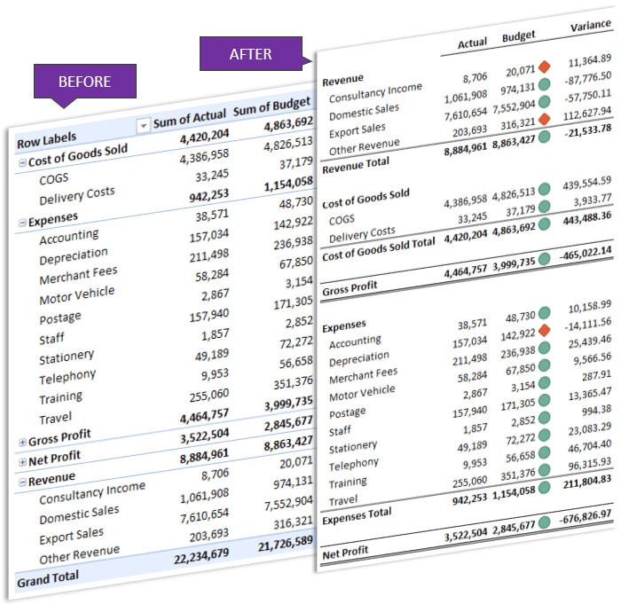
Pivot Table Before and after formatting

Table of Contents

  • Custom Sort Order
  • Column Labels
  • Inserting Blank Rows
  • Subtotal Position
  • Custom Styles
  • Conditional Formatting
  • Expand/Collapse Buttons
  • Repeating Item Labels
  • Report Layouts
  • Hiding (blank)s
  • Preserving Formatting
  • Default PivotTable Layout


Download PivotTable Formatting Cheat Sheet

Pivot table formatting cheat sheet

Enter your email address below to download the file.

By submitting your email address you agree that we can email you our Excel newsletter.
Please enter a valid email address.

Download the Cheat Sheet


Watch the Video

Subscribe YouTube

Custom Sort Order

By default, row and column labels are sorted alphabetically. We can use the built in sort options to sort based on a numeric field in ascending or descending order:

Pivot Table custom sort order

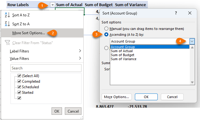
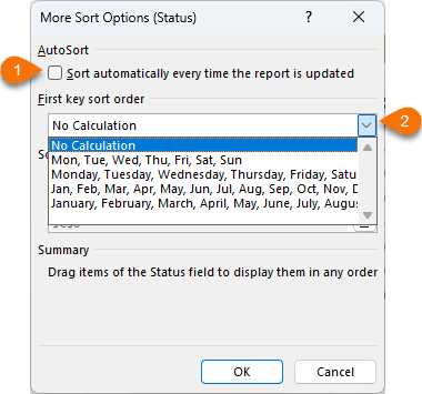
Or you can sort based on a custom list via the ‘More Options…’ button:

Pivot Table sort on custom list

However, often it’s quicker to sort by manually dragging the labels into place, or typing the label in the position you want it:

Manual sort in pivot table

Column Labels

By default, the column/row labels for the value fields are prefixed with ‘Sum of’, ‘Average of’ etc., which is often unnecessary, not to mention the helpful ‘Row Labels’ header, as you can see below:

Custom column labels for Pivot Table

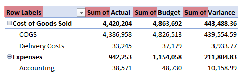
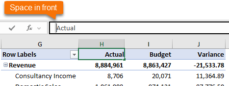
You can’t simply type ‘Actual’ in place of ‘Sum of Actual’ because this field name is already taken, however you can add a space in front or after ‘Actual’ to differentiate it. I like to add a space at the front so that I can right-align the column label in keeping with the numbers in the column below:

Add leading space to column label in Pivot Table

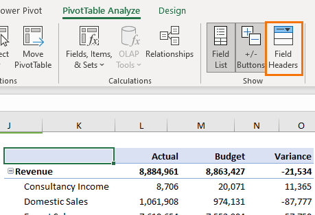
While you’re there, you can replace the ‘Row Labels’ header with a space in the cell to override it. Or, if you don’t want the filter drop down or the header, you can turn them both off by deselecting ‘Field Headers’ on the PivotTable Analyze tab:

Customize row header and field headers

Inserting Blank Rows

PivotTables can often look too busy and cramped. We can improve their readability by adding blank rows between each section:

add blank rows to Pivot Table

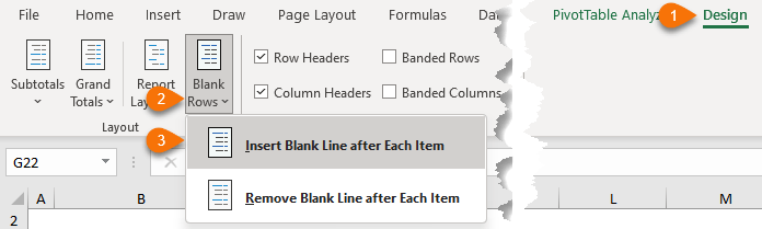
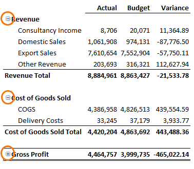
It immediately looks more like a Profit and Loss report, rather than a PivotTable:
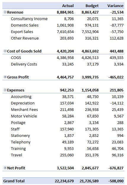
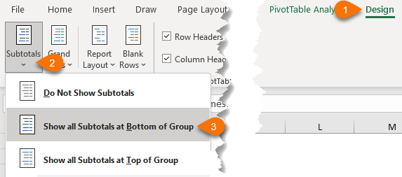
Pivot Table formatting like profit and loss statement

Subtotal Position

By default, subtotals are placed at the top of each section, however this may not always be appropriate. You can easily change the position to the bottom of the group:

Change position of subtotals in Pivot Table

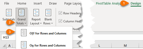
While I’m at it, I’ll also turn off the Grand Total row as it’s not required for this report:

turn off grand total row in pivot table

Custom Styles

It’s coming together but it still has that distinctive PivotTable formatting. We can remove that by creating a custom style that has no formatting.

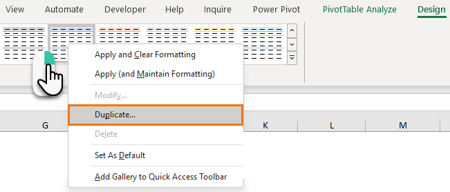
Duplicate any style by right-clicking on the thumbnail in the style gallery:

Duplicate Pivot Table style

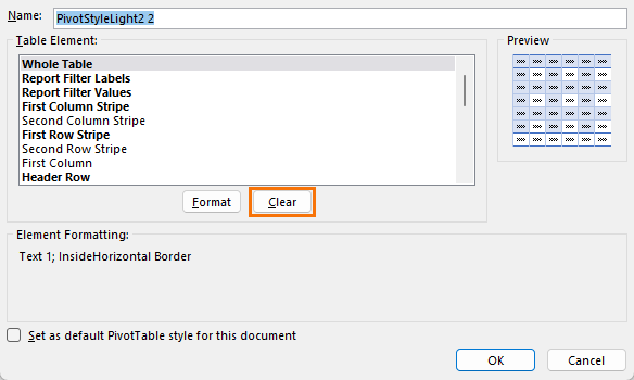
Then click ‘Clear’ for each of the elements in a bold font (the elements not in a bold font don’t have any formatting in that style):

clear bold formatting in Pivot Table style

Once you’ve created your custom style, don’t forget to apply it to your PivotTable by clicking on it in the Style Gallery.

Now that you have a blank canvas, you can select the elements in the PivotTable and apply the formatting you want.

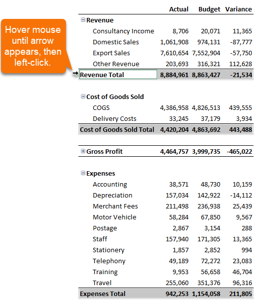
Tip: ensure you select the elements by clicking the left side (see image below) to select them all together, this way the format will be applied to the element, not the cells and if your PivotTable changes shape the format will follow the element:

Select element in Pivot Table style

Conditional Formatting

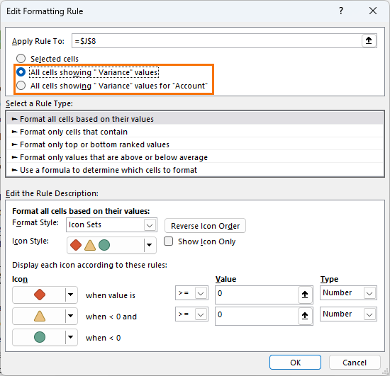
Adding visual indicators with conditional formatting can help your audience quickly interpret your reports. We can apply conditional formats to PivotTable value areas and have them automatically update when the PivotTable is refreshed by selecting one of the ‘all cells showing’ options:

Conditional formatting rule for Pivot Table

Step by step tutorial on conditional formatting PivotTables here.

Expand/Collapse Buttons

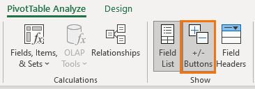
Expand and Collapse buttons enable you to quickly hide and unhide rows in the PivotTable:

Expand and collapse buttons for Pivot Table rows

If you don’t need the Expand/Collapse buttons, you can turn them off on the PivotTable Analyze tab:

turn off expand collapse buttons

Repeating Item Labels

When working with PivotTables in a Tabular layout, you may want to repeat the row labels for the purpose of using them in lookup formulas, or just for aesthetics.

repeating row labels in Pivot Table

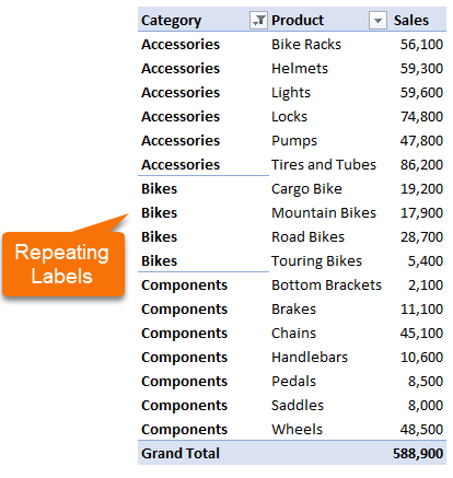
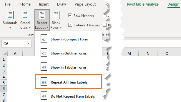
There are a few ways you can do this. You can turn it on for all item labels via the Design tab:

turn off repeating row labels in Design tab

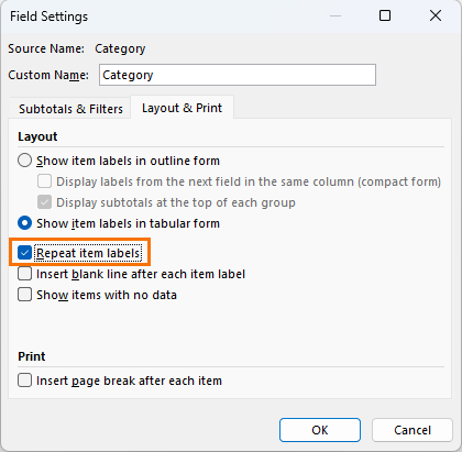
Or individually by right clicking on the field you want repeated > Field Settings > Layout & Print tab > Repeat item labels:

turn off repeating row labels in field settings

Report Layouts

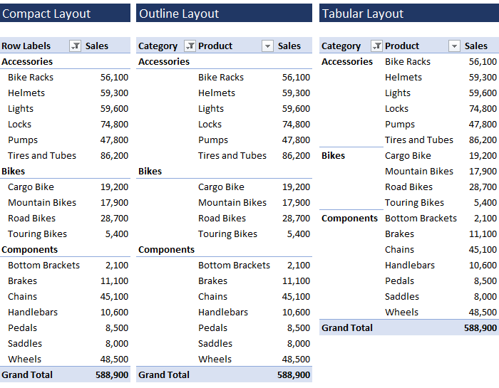
By default, PivotTables are created in compact form where row labels are nested, but we can also choose from an Outline layout or Tabular Layout:

choosing report layouts for a pivot table

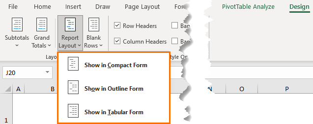
It’s quick and easy to change the layout via the Design tab:

change report layout for a pivot table

Hiding (blank)s

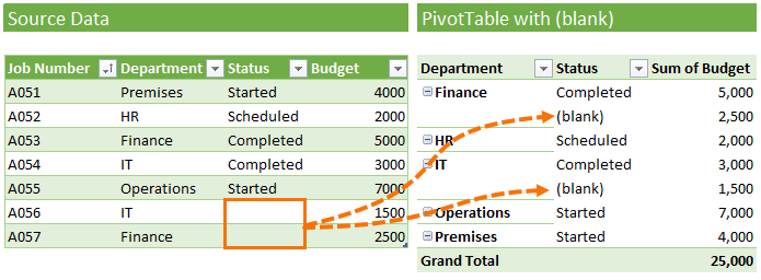
When you have blank cells in your source data, those blanks get labelled ‘(blank)’ in PivotTable row and column labels:

blank showing in a pivot table

Ideally you should never have blanks in columns that you use in row or column labels, but in the real world that’s not always possible, so the next best thing is to hide the blanks by selecting one of them and pressing the space bar > ENTER.

Formatting blanks in a pivot table

This needs to be done for each field in the PivotTable that contains blanks, but once applied, any new blanks that are added will not display (blank).

Another way is to hide blanks in PivotTables with Conditional Formatting.

This technique can be done once for all (blank) records, and therefore may be quicker if you have many fields with blanks.

Preserving Formatting

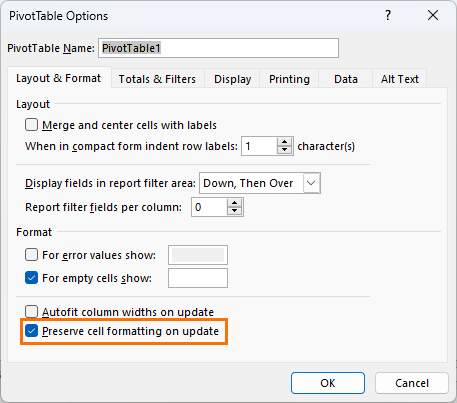
Once you’ve spent a load of time formatting your PivotTable, you’ll want to make sure that formatting sticks.

You can do this in the PivotTable Options (right click) > Layout & Format tab > Preserve cell formatting on update:

preserve cell formatting for a pivot table

Default PivotTable Layout

Once you’ve got the formatting the way you like it, you can set a default PivotTable layout via the File tab > Options:

set pivot table default layout

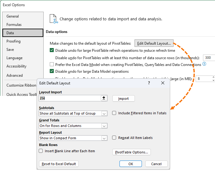
You can set preferences for the subtotals, grand totals, report layout, blank rows and PivotTable Options. Unfortunately, you can’t set preferences for number formats or styles.


PivotTable Formatting
Mynda Treacy

Microsoft MVP logo

AUTHOR Mynda Treacy Co-Founder / Owner at My Online Training Hub

CIMA qualified Accountant with over 25 years experience in roles such as Global IT Financial Controller for investment banking firms Barclays Capital and NatWest Markets.

Mynda has been awarded Microsoft MVP status every year since 2014 for her expertise and contributions to educating people about Microsoft Excel.

Mynda teaches several courses here at MOTH including Excel Expert, Excel Dashboards, Power BI, Power Query and Power Pivot.

More Excel PivotTables Posts

Images in Excel Pivot Tables

Images in Excel PivotTables

Include images in Excel PivotTables, combined with some slick formatting, and create dynamic and visually rich PivotTables like never before.

Auto Refresh PivotTables

Auto Refresh PivotTables isn’t on by default, and the process differs depending on if your PivotTables is loaded to the data model or not.

Show Items with no Data in PivotTables

Show Items with no Data in PivotTables allows you to maintain a constant structure to your PivotTable or Pivot Chart axis when filtering.

Force Excel Slicers to Single Select

There's no build in way to force Excel Slicers to single select but we can use these clever warnings to persuade your users.
excel pivottable p&L

Excel PivotTable Profit and Loss

Creating an Excel PivotTable Profit and Loss Statement means you can use Slicers and Conditional Formatting and have the P&L automatically update.

Excel PivotTable Field List Tips

Customize the Excel PivotTable Field List to suit your needs. Find how to turn the PivotTable Field List on and off and other handy tips.

Hide Blanks in Excel PivotTables

Hide blanks in Excel PivotTables caused by empty cells in your source data. I’m talking about PivotTable cells containing the (blank) placeholder.
Excel Slicer Formatting

Excel Slicer Formatting

Excel Slicer Formatting is essential because they’re big and chunky. In this tutorial I show you the tricks to make Excel Slicers small.
Excel PivotTable Quick Explore

Excel PivotTable Quick Explore

Drill down into data hierarchies using PivotTables and Pivot Charts with Excel PivotTable Quick Explore. New in Excel 2013 onward.
excel online pivottables

Excel Online PivotTables

Excel Online PivotTables are now available from the Insert tab of the ribbon. There are some limitations that are covered in this post.


Category: Excel PivotTables
Previous Post:Images in Excel Pivot TablesImages in Excel PivotTables
Next Post:Pro Excel Chart Formattingprofessional vs amateur chart formatting

Reader Interactions

Comments

  1. Floyd Henry

    September 8, 2023 at 1:31 am

    A wonderful tool to use to make formatting of even complex pivot tables easy.
    Thank you so much

    Floyd Henry,
    Director, Quality Assurance

    Reply
    • Mynda Treacy

      September 8, 2023 at 8:57 am

      Our pleasure, Floyd!

      Reply
  2. Anthony

    August 17, 2023 at 2:05 am

    Hi, thanks very much for the article however I have a big problem with this.

    Even with “Preserve cell formatting on update” selected, every time the Pivot table is updated the formatting is lost. This includes changing the order of a field in Rows section or swapping a column or pressing “Refresh”. So all the hard work creating a custom layout is lost.

    This issue is also mentioned here as just one example: https://techcommunity.microsoft.com/t5/excel/pivot-table-formatting-after-refresh/m-p/510256

    Any ideas?
    Many thanks,
    Anthony

    Reply
    • Mynda Treacy

      August 17, 2023 at 10:28 am

      Hi Anthony,

      Formatting vs row/column order are different issues. It sounds like the source data is changing on refresh, affecting the sorting of the items and fields. Is that possible?

      Mynda

      Reply
      • souleymane

        September 8, 2023 at 9:00 am

        Hi Mynda how to get data of this example i whant to pratics

        Reply
        • Mynda Treacy

          September 8, 2023 at 9:41 am

          It’s available from the PivotTable Profit and Loss tutorial.

          Reply

Leave a Reply Cancel reply

Your email address will not be published. Required fields are marked *

Current ye@r *

Leave this field empty

Sidebar

More results...

Popular Content

  • 10 Common Excel Mistakes to Avoid
  • Top Excel Functions for Data Analysts
  • Secrets to Building Excel Dashboards in Less Than 15 Minutes
  • Pro Excel Formula Writing Tips
  • Hidden Excel Double-Click Shortcuts
  • Top 10 Intermediate Excel Functions
  • 5 Pro Excel Dashboard Design Tips
  • 5 Excel SUM Function Tricks
  • 239 Excel Keyboard Shortcuts

100 Excel Tips and Tricks eBook

Download Free Tips & Tricks

239 Excel Keyboard Shortcuts

Download Free PDF

mynda treacy microsoft mvpHi, I'm Mynda Treacy and I run MOTH with my husband, Phil. Through our blog, webinars, YouTube channel and courses we hope we can help you learn Excel, Power Pivot and DAX, Power Query, Power BI, and Excel Dashboards.

Blog Categories

  • Excel
  • Excel Charts
  • Excel Dashboard
  • Excel Formulas
  • Excel Office Scripts
  • Excel PivotTables
  • Excel Shortcuts
  • Excel VBA
  • General Tips
  • Online Training
  • Outlook
  • Power Apps
  • Power Automate
  • Power BI
  • Power Pivot
  • Power Query
microsoft mvp logo
trustpilot excellent rating
Secured by Sucuri Badge
MyOnlineTrainingHub on YouTube Mynda Treacy on Linked In Mynda Treacy on Instagram Mynda Treacy on Twitter Mynda Treacy on Pinterest MyOnlineTrainingHub on Facebook

Sign up to our newsletter and join over 400,000
others who learn Excel and Power BI with us.


Company

  • About My Online Training Hub
  • Disclosure Statement
  • Frequently Asked Questions
  • Guarantee
  • Privacy Policy
  • Terms & Conditions
  • Testimonials
  • Become an Affiliate
  • Sponsor Our Newsletter

Support

  • Contact
  • Forum
  • Helpdesk – For Technical Issues

Copyright © 2023 · My Online Training Hub · All Rights Reserved. Microsoft and the Microsoft Office logo are trademarks or registered trademarks of Microsoft Corporation in the United States and/or other countries. Product names, logos, brands, and other trademarks featured or referred to within this website are the property of their respective trademark holders.

Download A Free Copy of 100 Excel Tips & Tricks

excel tips and tricks ebook

We respect your privacy. We won’t spam you.

x