Set Excel PivotTable Default Layout

New in Excel 2019 onward and Microsoft 365 is the ability to set a PivotTable default layout, which can save a load of time.

If you’re like many PivotTable users the first thing you do after inserting a PivotTable is waste a minute or so fixing the layout so it’s just how you want.  Waste no more, because now you can set the default for any new PivotTables in any workbook.

Setting a default PivotTable layout doesn’t change or update existing PivotTables though.

Watch the Video

How to Set Excel PivotTable Default Layout

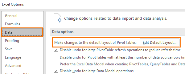
You’ll find the settings for the default PivotTable layout in the Options: File tab > Options > Data > Edit Default Layout:

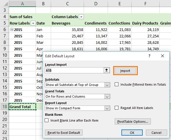
You can import a layout from an existing PivotTable; just select a cell in the PivotTable and click ‘Import’:

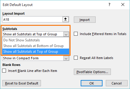
Or you can specify the layout for the Subtotals:

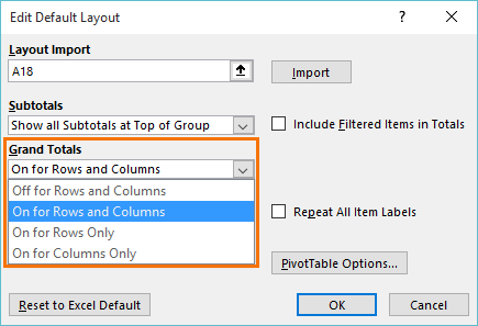
The Grand Totals:

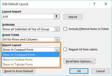
The Report Layout:

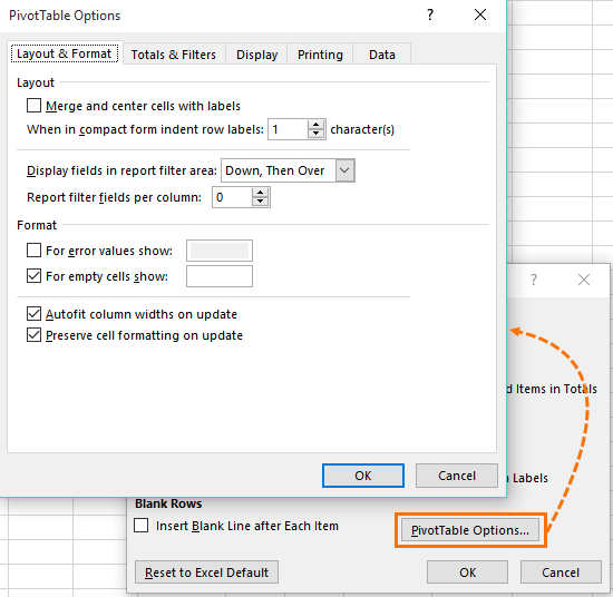
Even the PivotTable Options:

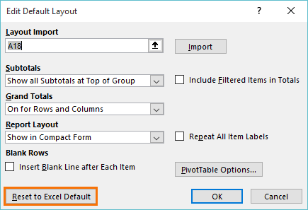
And if you get tired of your default layout, you can restore the Excel default:

Note: the default layout only applies to the current workbook. If you want to have these defaults in every new workbook then you can customize your default workbook.

PivotTable Default Styles

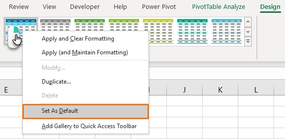
Unfortunately, the styles aren't part of the default PivotTable layout settings, however they're easy to set. Simply right-click the style in the gallery that you want as your default and select 'Set as default':

PivotTable Default Number Formats

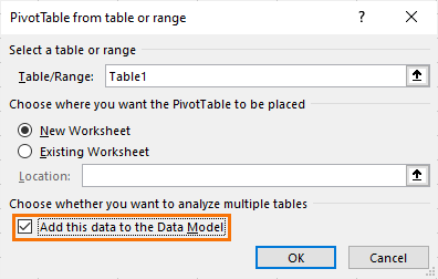
With regular PivotTables there's no way to set the default number format for a field. However, with Power Pivot we can. Simply add your data to the Data Model when creating the PivotTable:

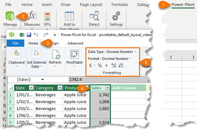
Then open the Power Pivot window, select the column you want to format and on the Home tab set the number format:

Note: there are some knock on effects when adding data to the data model:

First, the GETPIVOTDATA function references are slightly different.

When you reference a value cell in a Power Pivot PivotTable the references contain the word ‘Measures’ and the table and column names are included, as you can see below:

=GETPIVOTDATA("[Measures].[Sum of Sales]",$A$3,"[Table1].[Category]","[Table1].[Category].&[Beverages]","[Table1].[Product]","[Table1].[Product].&[Chai]")

Whereas when you reference a value field in a regular PivotTable, Measures doesn’t appear, and the references are simply the field names and items like this:

=GETPIVOTDATA("Sales",$E$21,"Category","Beverages","Product","Chai")

These differences aren’t really an issue, but if you want to create dynamic GETPIVOTDATA formulas then you need to allow for this.

• GETPIVOTDATA function for regular PivotTables
• GETPIVOTDATA function for data model/Power Pivot PivotTables

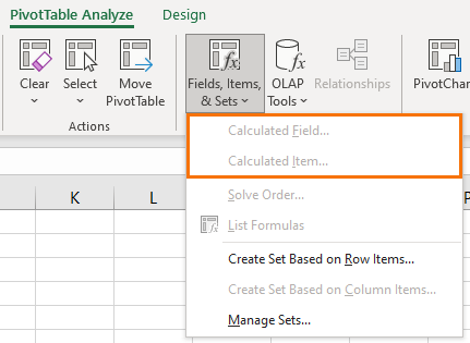
The other main difference is that you no longer have access to the calculated fields and columns functionality we have with regular PivotTables. You’ll notice they're greyed out in the menu:

Instead, with Power Pivot we must add calculated columns in the Power Pivot window using the DAX formula language. And calculated items are measures, which are also written with DAX. The good thing is the DAX formula language is very similar to the Excel functions we know and love. If you’d like to learn DAX, please check out my Power Pivot course which covers DAX.

Bonus for OLAP PivotTables

Tip: a recent performance improvement to Excel 2019 onward means that disabling Subtotals and Grand Totals can make OLAP PivotTables faster.

Non Microsoft 365 Users

If you don’t have the latest version of Excel then there are still some one-click shortcuts to making some of the more common changes to PivotTable layouts. Namely, removing all subtotals and reinstating the ‘classic PivotTable’ layout, which is tabular, as described in this post.