• Skip to main content
  • Skip to header right navigation
  • Skip to site footer

My Online Training Hub

Learn Dashboards, Excel, Power BI, Power Query, Power Pivot

  • Courses
  • Pricing
    • Free Courses
    • Power BI Course
    • Excel Power Query Course
    • Power Pivot and DAX Course
    • Excel Dashboard Course
    • Excel PivotTable Course – Quick Start
    • Advanced Excel Formulas Course
    • Excel Expert Advanced Excel Training
    • Excel Tables Course
    • Excel, Word, Outlook
    • Financial Modelling Course
    • Excel PivotTable Course
    • Excel for Customer Service Professionals
    • Excel for Operations Management Course
    • Excel for Decision Making Under Uncertainty Course
    • Excel for Finance Course
    • Excel Analysis ToolPak Course
    • Multi-User Pricing
  • Resources
    • Free Downloads
    • Excel Functions Explained
    • Excel Formulas
    • Excel Add-ins
    • IF Function
      • Excel IF Statement Explained
      • Excel IF AND OR Functions
      • IF Formula Builder
    • Time & Dates in Excel
      • Excel Date & Time
      • Calculating Time in Excel
      • Excel Time Calculation Tricks
      • Excel Date and Time Formatting
    • Excel Keyboard Shortcuts
    • Excel Custom Number Format Guide
    • Pivot Tables Guide
    • VLOOKUP Guide
    • ALT Codes
    • Excel VBA & Macros
    • Excel User Forms
    • VBA String Functions
  • Members
    • Login
  • Blog
  • Excel Webinars
  • Excel Forum
    • Register as Forum Member

Hide Blanks in Excel PivotTables

You are here: Home / Excel PivotTables / Hide Blanks in Excel PivotTables
October 11, 2018 by Mynda Treacy

There are a couple of ways you can hide blanks in Excel PivotTables. To be clear, the ‘blanks’ I’m referring to are those shown below where the text, (blank), is inserted as a placeholder for empty cells in your source data:

hide blanks in Excel PivotTables

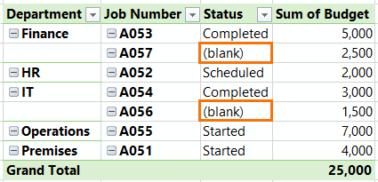
It’s important to point out that these (blank) placeholders only occur in row or column areas, and never in the values area of a PivotTable.

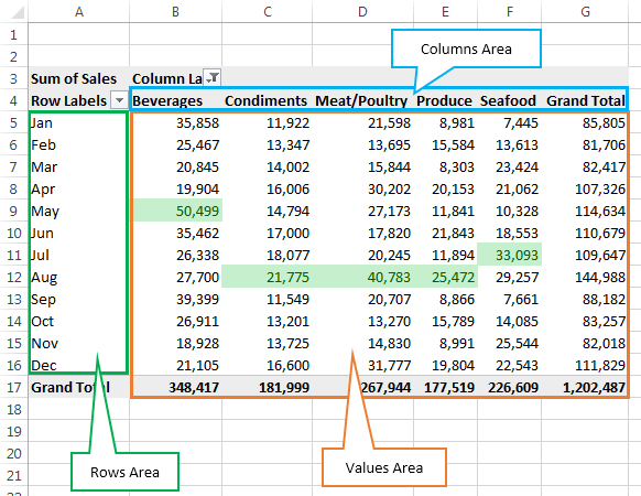
Here’s a diagram so you know what I mean by the different areas of a PivotTable:

sum of sales

The Cause of (blank) in PivotTables

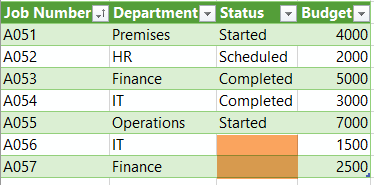
The (blank) placeholder is caused by empty cells in your source data, like those shown in the Status column of my source data below:

blanks

How to Hide (blank) in PivotTables

Option 1: Ideally your source data shouldn’t have any blank or empty cells. So, the best solution to hide blanks in Excel PivotTables is to fill the empty cells. However, this isn’t always practical, hence options 2 and 3 below.

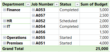
Option 2: Select any single cell in the PivotTable that contains (blank) and enter a space in the cell. Like magic it will replace all (blank) values for that field with a space, which is more aesthetically pleasing:

replace all blank values

Pros: This setting is automatically applied to any new data added to your source that also contains empty cells. And if you add data to cells in your source data that were previously blank, the PivotTable will correctly update. i.e. the cells containing the space will be replaced with the new data upon refreshing the PivotTable.

Cons: If you have multiple fields containing blanks e.g. Department and Status, then you need to repeat this for each field. No biggy.

Option 3: Conditional Formatting can be used to hide the (blank) text.

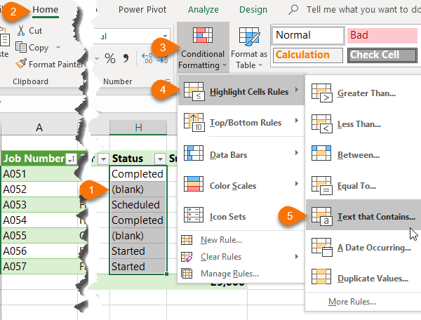
Steps (as shown in the image below):

  1. Select the cells (PivotTable column or rows) containing (blank)
  2. Home tab
  3. Conditional Formatting
  4. Highlight Cells Rules
  5. Text that Contains…

conditional formatting to hide pivottable blanks

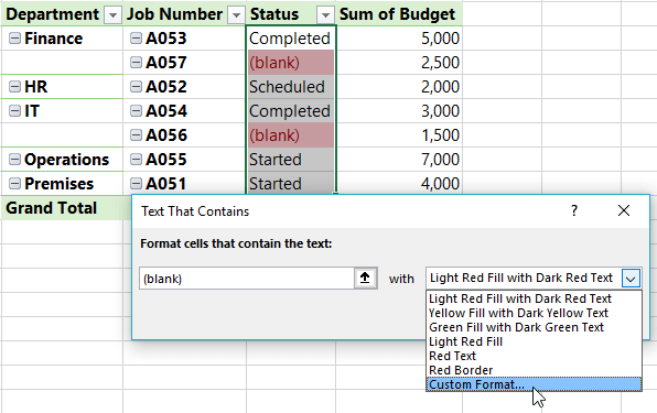
In the dialog box (shown below) enter ‘(blank)’ and select ‘Custom Format…’ from the drop-down list:

select custom format from the drop down

In the Format Cells dialog box choose ‘Custom’ in the ‘Category’ list on the ‘Number’ tab, and in the ‘Type’ field enter 3 semi-colons:

enter 3 semi-colons

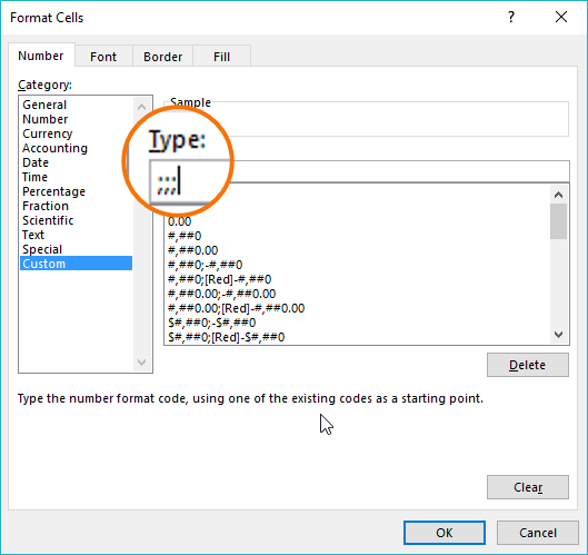
The 3 semi-colons simply tell Excel to hide all text or numbers in the cell, and the Conditional Formatting rule restricts this format to only those cells that contain the text ‘(blank)’.

Tip: Learn more about Excel Custom Number formats here.

Pros: It hides the (blank) placeholder and once the empty cells in the source data contain text or values they no longer meet the condition, so the actual text or values are displayed.

Cons: Requires manual updating if the PivotTable grows. Alternatively, you can apply the Conditional Formatting to the whole column/row. However, if your PivotTable changes shape, you’ll need to update the range the Conditional Format is applied to. This can be done via the Home tab > Conditional Formatting > Manage Rules dialog box:

manage rules dialog box

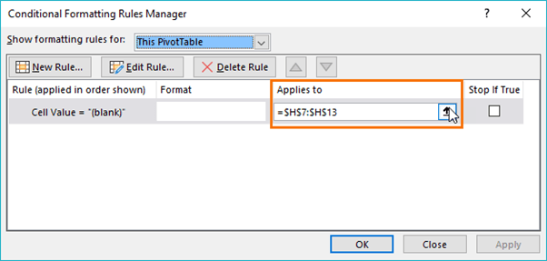
This is because Conditional Formatting applied to row or column labels doesn’t automatically adapt to changes in the PivotTable shape or size, unlike when applied to the values area.

Personally, I like option 2 because it’s easier. You can call me lazy, but I like to call it efficient 😉

Download the Workbook

Enter your email address below to download the sample workbook.

By submitting your email address you agree that we can email you our Excel newsletter.
Please enter a valid email address.

Download the Excel Workbook. Note: This is a .xlsx file please ensure your browser doesn't change the file extension on download.

More Excel PivotTable Posts

show report filter pages for power pivot pivottables

Show Report Filter Pages for Power Pivot PivotTables

PivotTables created from Power Pivot can't use the 'Show Report Filter Pages' option. But this piece of VBA allows you to do just that.
Conditional Formatting PivotTables

Conditional Formatting PivotTables

Conditional Formatting PivotTables values areas will automatically expand/contract as you add new data or make changes to the filters, rows or columns.
Display Missing Dates in Excel PivotTables

Display Missing Dates in Excel PivotTables

Filter Excel Pivot Tables by Values

Filter Excel Pivot Tables by Values

Excel PivotTable Month Comparison [Video]

Excel PivotTable Month Comparison [Video]

Excel PivotTable Month Comparison is easy with the Show Values As tool.
Excel PivotTable Add Percentage of Total Column [Video]

Excel PivotTable Add Percentage of Total Column [Video]

Excel PivotTable Add Percentage of Total Column is easy via the Show Values As settings.
Excel Factor 6 Auto Refresh PivotTables

Excel Factor 6 Auto Refresh PivotTables

Excel Factor Entry 1 - Reverse PivotTable

Excel Factor Entry 1 – Reverse PivotTable

More Excel PivotTables Posts

Auto Refresh PivotTables

Auto Refresh PivotTables isn’t on by default, and the process differs depending on if your PivotTables is loaded to the data model or not.

Show Items with no Data in PivotTables

Show Items with no Data in PivotTables allows you to maintain a constant structure to your PivotTable or Pivot Chart axis when filtering.

Force Excel Slicers to Single Select

There's no build in way to force Excel Slicers to single select but we can use these clever warnings to persuade your users.
excel pivottable p&L

Excel PivotTable Profit and Loss

Creating an Excel PivotTable Profit and Loss Statement means you can use Slicers and Conditional Formatting and have the P&L automatically update.

Excel PivotTable Field List Tips

Customize the Excel PivotTable Field List to suit your needs. Find how to turn the PivotTable Field List on and off and other handy tips.

Hide Blanks in Excel PivotTables

Hide blanks in Excel PivotTables caused by empty cells in your source data. I’m talking about PivotTable cells containing the (blank) placeholder.
Excel Slicer Formatting

Excel Slicer Formatting

Excel Slicer Formatting is essential because they’re big and chunky. In this tutorial I show you the tricks to make Excel Slicers small.
Excel PivotTable Quick Explore

Excel PivotTable Quick Explore

Drill down into data hierarchies using PivotTables and Pivot Charts with Excel PivotTable Quick Explore. New in Excel 2013 onward.
excel online pivottables

Excel Online PivotTables

Excel Online PivotTables are now available from the Insert tab of the ribbon. There are some limitations that are covered in this post.

Excel PivotTable Error Handling

Excel PivotTable error handling and why you can’t calculate the percentage change when the prior period is zero or blank.


Category: Excel PivotTablesTag: Excel PivotTable
Previous Post:Excel Data TypesExcel Data Types
Next Post:Web Scraping With VBAweb scraping with vba

Reader Interactions

Comments

  1. Cooper

    October 28, 2020 at 12:20 pm

    How to hide blank values and blank rows in Top 20 PivotTables?

    Thank you.

    Reply
    • Mynda Treacy

      October 28, 2020 at 8:01 pm

      Hi Cooper, you can filter out blanks using the filter buttons on the PivotTable column headers. Hiding blanks is explained in the tutorial above. Mynda

      Reply
  2. Claudine

    February 14, 2020 at 1:30 am

    Option 2 is great indeed

    Rirst time today that I experience it’s not working on some of my fields. Is there any know reason when this could happen?

    Kr Claudine

    Reply
    • Mynda Treacy

      February 14, 2020 at 10:38 am

      Hi Claudine, I can’t think of a reason for it not to work. You’re welcome to share your Excel file on our forum and we can take a look for you.

      Reply
  3. Kamran Mumtaz

    November 7, 2019 at 9:59 pm

    Hi, I wanna get rid of entire rows that have blanks or zeros…?

    Reply
    • Mynda Treacy

      November 8, 2019 at 9:30 am

      You can use the Filters (drop down buttons on the PivotTable) to filter out blanks for specific columns/rows.

      Reply
  4. nj s27

    September 8, 2019 at 11:01 am

    Is there an easy vba solution for this?

    Reply
    • Philip Treacy

      September 8, 2019 at 1:04 pm

      why use VBA?

      Reply
  5. Joan

    October 12, 2018 at 8:03 am

    Nice!

    Reply
    • Mynda Treacy

      October 12, 2018 at 8:09 am

      Glad you liked it, Joan 🙂

      Reply
  6. Danny Eisenbacher

    October 12, 2018 at 3:37 am

    For method 3, can’t you just increase the “applies to” range to a much larger area? Then as the pivot table increases, it will still be applying it to the new area. For this example, it could be applied to $F$1:$H$1000 so that as more rows are added to the pivot table it would continue to be updated. After it is applied in this manner, Excel breaks the applied to range to the region before the pivot table, the region after the pivot table, and the region in the table. It does automatically update those regions as the pivot table is refreshed.

    Reply
    • Mynda Treacy

      October 12, 2018 at 8:45 am

      Hi Danny,

      Yes, I eluded to increasing the Conditional Formatting range in step 3, but it’s not recommended to apply formatting to a bigger range than you need as this can have performance repercussions. For small ranges it’s not an issue, but you don’t want to be applying it to large areas. Also, if you continue to make changes to your PivotTable layout the Conditional Format ‘Applies to’ range becomes very messy.

      It’s just not best practice, and option 2 is dead easy, so I recommend that approach.

      Mynda

      Reply

Leave a Reply Cancel reply

Your email address will not be published. Required fields are marked *

Current ye@r *

Leave this field empty

Sidebar

More results...

launch excel macros course excel vba course

Featured Content

  • 10 Common Excel Mistakes to Avoid
  • Top Excel Functions for Data Analysts
  • Secrets to Building Excel Dashboards in Less Than 15 Minutes
  • Pro Excel Formula Writing Tips
  • Hidden Excel Double-Click Shortcuts
  • Top 10 Intermediate Excel Functions
  • 5 Pro Excel Dashboard Design Tips
  • 5 Excel SUM Function Tricks
  • 239 Excel Keyboard Shortcuts

100 Excel Tips and Tricks eBook

Download Free Tips & Tricks

Subscribe to Our Newsletter

Receive weekly tutorials on Excel, Power Query, Power Pivot, Power BI and More.

We respect your email privacy

239 Excel Keyboard Shortcuts

Download Free PDF

mynda treacy microsoft mvpHi, I'm Mynda Treacy and I run MOTH with my husband, Phil. Through our blog, webinars, YouTube channel and courses we hope we can help you learn Excel, Power Pivot and DAX, Power Query, Power BI, and Excel Dashboards.

Blog Categories

  • Excel
  • Excel Charts
  • Excel Dashboard
  • Excel Formulas
  • Excel PivotTables
  • Excel Shortcuts
  • Excel VBA
  • General Tips
  • Online Training
  • Outlook
  • Power Apps
  • Power Automate
  • Power BI
  • Power Pivot
  • Power Query
microsoft mvp logo
trustpilot excellent rating
Secured by Sucuri Badge
MyOnlineTrainingHub on YouTube Mynda Treacy on Linked In Mynda Treacy on Instagram Mynda Treacy on Twitter Mynda Treacy on Pinterest MyOnlineTrainingHub on Facebook
 

Company

  • About My Online Training Hub
  • Disclosure Statement
  • Frequently Asked Questions
  • Guarantee
  • Privacy Policy
  • Terms & Conditions
  • Testimonials
  • Become an Affiliate

Support

  • Contact
  • Forum
  • Helpdesk – For Technical Issues

Copyright © 2023 · My Online Training Hub · All Rights Reserved. Microsoft and the Microsoft Office logo are trademarks or registered trademarks of Microsoft Corporation in the United States and/or other countries. Product names, logos, brands, and other trademarks featured or referred to within this website are the property of their respective trademark holders.