Creating an Excel PivotTable Profit and Loss statement is surprisingly easy. And because it’s a PivotTable you can team it with Slicers to make it interactive.
While you’re at it you might as well add some conditional formatting to make reading, what is usually a drab report, quick and easy.
Watch the Video

Download Template Workbook
Enter your email address below to download the sample workbook.

Excel PivotTable Profit and Loss Step by Step Instructions
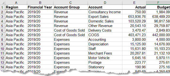
My data (shown below) is in a tabular layout with each account classified into an ‘Account Group’. These account groups represent the different sections of a Profit and Loss statement.
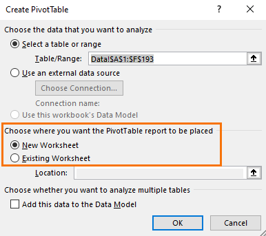
Step 1: Insert a PivotTable
Select the data > Insert tab > PivotTable. In the dialog box choose whether you want it in a new sheet or existing sheet.
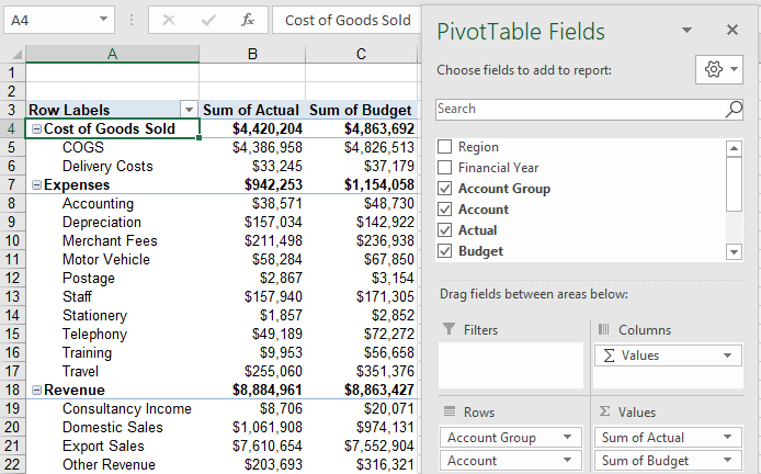
Step 2: Build the PivotTable
Add the Account Group and Account fields to the Rows and add Actual and Budget to the Values:
Step 3: Rearrange the Account Group order
The Revenue accounts should be listed first, then Cost of Goods Sold, then Expenses. Left click and drag Revenue to the top of the row labels area:
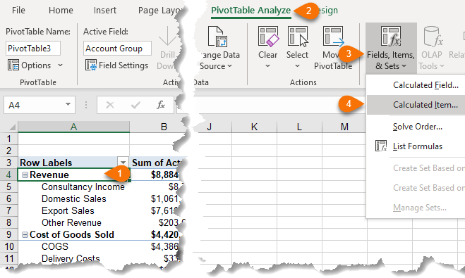
Step 4: Add Calculated Items for Gross Profit and Net Profit
Select one of the Account Group cells in the row labels area of the PivotTable > PivotTable Analyze tab > Fields, Items & Sets > Calculated Item:
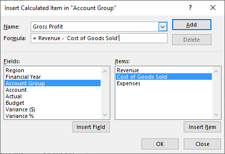
We’ll create the Gross Profit item first:
Then one for Net Profit:
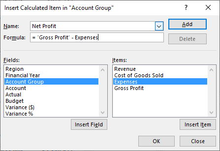
They should now appear in the PivotTable row labels.
Step 5: Collapse the Gross Profit and Net Profit Items
This hides the underlying account detail that makes up these values:
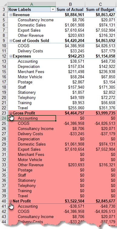
Also move Gross Profit up under Cost of Goods Sold using the left click and drag technique covered in step 3.
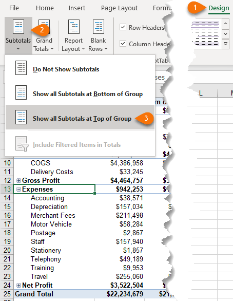
Step 6: Show Subtotals at Bottom of Group
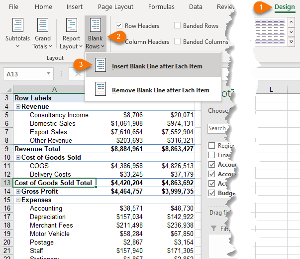
Step 7: Insert Blank Line after Each Item
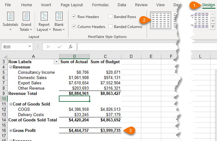
Step 8: Format PivotTable
Choose a plain style from the gallery on the Design tab or create your own with no formatting, as I’ve done for this example. Then add cell borders for the sub-total and total rows:
Make sure ‘Preserve cell formatting on update’ is on by right clicking the PivotTable > PivotTable Options > Layout & Format tab:
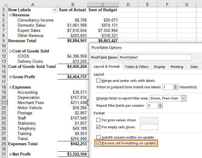
Rename the Actual and Budget headings to remove the ‘Sum of’ by replacing them with a space. We need to add the space at the front of the labels because we cannot use names that are also in the field list.
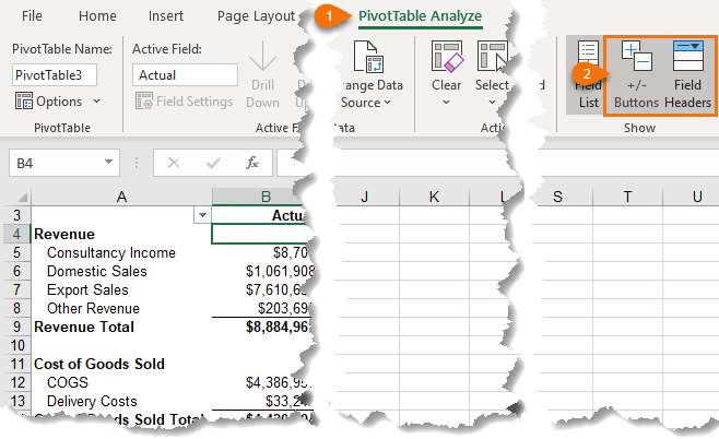
Hide the Expand and Collapse buttons and Field Headers:
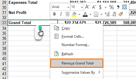
Remove the Grand Total: right click the Grand Total label > Remove Grand Total:
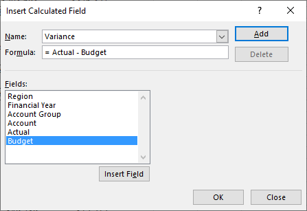
Step 9: Add a Calculated Field for the Variance (Optional)
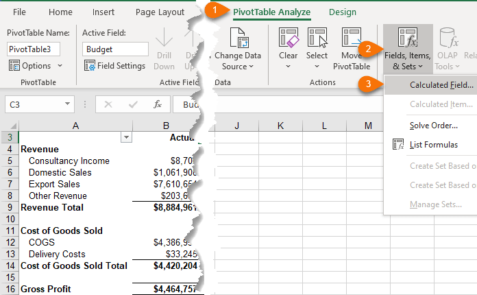
In the formula field subtract the budget from the actual:
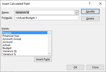
You can also add one for the % Variance if you want:
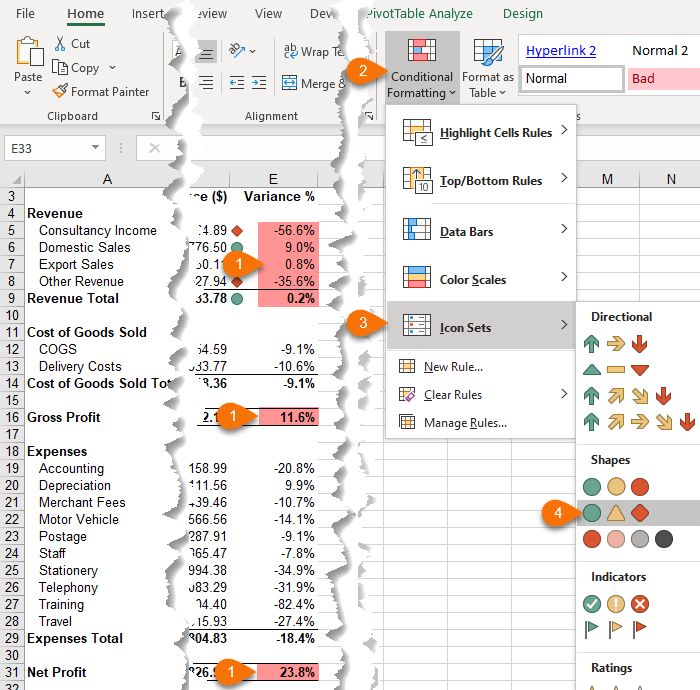
Step 10: Conditional Formatting (Optional)
Profit and loss statements make for dry reading, but we can make it quicker for our audience to interpret with the help of some conditional formatting to visually indicate whether the variance is positive or negative using traffic lights.
Positive income variances are good, but the opposite is true for expense variances, so we need two conditional formatting rules.
Set up the income rule first by selecting just the income related Variance % cells: Revenue, Gross Profit and Net Profit > Home tab > Conditional Formatting > Icon Sets:
Repeat for the Cost of Goods Sold and Expenses Variance % cells.
Modify the Conditional Formatting rules: Home tab > Conditional Formatting > Manage Rules…
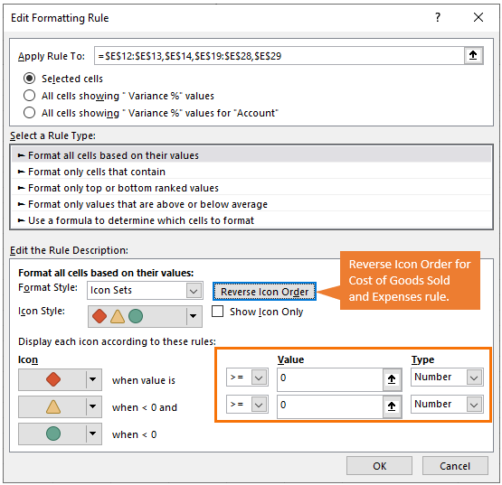
Select each rule and edit them as per the settings below:
Step 11: Add Slicers (Optional)
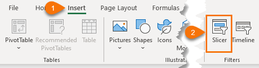
If your source data has fields that you’d like to filter your Profit and Loss by, you can add Slicers by selecting a cell in the PivotTable > Insert tab > Slicers
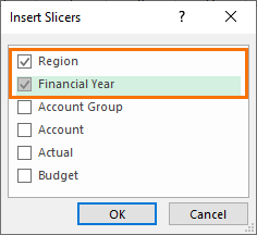
I’ll add them for Region and Financial Year:
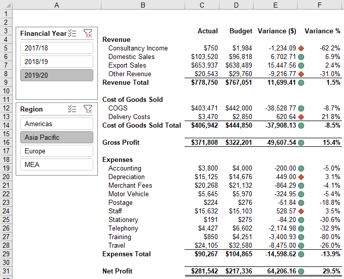
And your PivotTable Profit and Loss is done:

Thanks for this clear presentation. Please assist with similar presentation of an FS (Income Statement & Balance Sheet) using Trial Balance as the data reference.
Glad you found it useful, Rabiu. You can use the same techniques to build your other financial statements.
Mynda,
I’m a big fan and have taken a couple of your courses.
Your P&L looks great! I’m trying to create one with formatting that is automatically adjusted when there are more or fewer items in each category. Any suggestions?
Great to hear, Brian! You can use Conditional Formatting to identify rows that are ‘totals’ and rows that aren’t and apply the formatting accordingly. If you get stuck, please post your question on our Excel forum where you can also upload a sample file and we can help you further.
GREAT job as always!
I laugh when I looked at the P/L b/e I was hired as a consultant to do this but could not find ANYTHING on doing this through DAX; and mightily struggled. NOW, in your model the 1st income line is “Consultancy Income” – and YOU have it! Where were you 5 yrs ago! Things, and teachings are always improving!
(And I will be going through this in minute detail!)
Have a Merry Christmas down in OZ!
😀 so glad it will be useful to you, Merrill! Merry Christmas to you too!
Can you order the Accounts shown under the major groupings in a particular way other than alphabetically?
Yes, you can simply left click and drag the outer edge of the row label cell to a new position 🙂
Hi Mynda,
I am trying to calculate the GP%, but had no luck. Any reason why this does not work. I used GP/Revenue. Thanks Marlon
Hard to say without seeing your file. Please post your question on our Excel forum where you can also upload a sample file and we can help you further.
I was using your sample file used above for the GP% calculation.
Thanks
Marlon
Oh, ok. Because the Gross Profit is actually the sum of the accounts that make up the revenue and COGS account groups, as opposed to a calculation in its own right. If you turn the field buttons back on and expand the Gross Profit line, you’ll see the underlying accounts that make it up. It’s just a limitation of regular PivotTables, I’m afraid.
Hi Myanda,
Earlier this week, I was asked by a Manager to draw up a P&L for a Camp ( Resort ) and after searching “hi&lo” for a “how to create a P&L in a pivot table” tutorial, I stumbled on this from 2020 ..
.. it was exactly what I needed !!
I had to tweak the “calculated items” formulas for Gross & Net Profit as our Company shows revenue as ( – ), but aside from that, and a couple of revenue variance ( % ) that seem odd, I’m very happy with the result.
So pleased to hear that, John!
Dear Teacher
I am 68 and never learned so fast in my life, I must say you are the best teacher and I salute you for it.
Be Blessed
Rathod
Wow, that’s amazing to hear, Rathod! Thank you for your kind words. Never stop learning 🙂
Very helpful, indeed you are a teacher.
Have you covered the ones involving trial balance and balance sheet? Do you also have as any tutorial on macros and VBA?
Hi Anyim,
No, I haven’t done any on trial balance and balance sheet. A trial balance should be straight forward, and the Balance Sheet will use the same techniques used here. You can find all our VBA tutorials here: https://www.myonlinetraininghub.com/category/excel-vba
Mynda
Do you have any tutorial how to create P/L using power Pivot, I have my normalized tables in SQL Server, wondering how to do using DAX . Thank you.
Hi Giovanni,
No, I don’t have any Power Pivot P&L tutorials. It’s notoriously difficult to create them with Power Pivot.
Mynda
Hi Tracy,
When I insert the Calculated Items to get the Revenue mins Expense, the Excel show “This PivotTable report field is grouped. You cannot add a calculated item to a grouped field.”
Can you please advise what went wrong? How can I fix this?
Thanks a lot.
Christina
Hi Christina,
Sounds like a field in your Pivot Table or cache is grouped. Most likely the date field. Right-click on the fields > ungroup.
Mynda
Hello,
Could you confirm that OR we have Calculated Items OR we have goruped Dates (year, moth, day).
Is there any turn around?
Thanks
HI
In between I found a turn around. In Power Wuery, created colluns from Data collun with year, month wuarter, wee, and voila.
Thanks. I want to use this opportunity to cangratulate you for your videos and material. They are superb. I’m planning to role in your Courses, but for now I want to see what I can do before I use my year with “you” to go deeper.
Thanks
Rui
Glad you found a solution, Rui!
Hi Mynda,
I watched your webinar training how to create interactive dashboard and it is excellent. I was able to create my own Sales Order dashboard with your excellent tools and input from the webinar using one big data information. My boss really loves it and he wanted me to add more information using the same dashboard. Unfortunately, the additional information is a totally separate set of data. Am I able to combine two or three sets of data in one dashboard?
Great to hear my tutorial was helpful. If you want to work with multiple datasets you can either consolidate them all into one table using Power Query, or use Power Pivot to create a model and related tables that can then be summarised in the same PivotTable.
Dear Mynda
Simply wonderful!
By the end of the week, I hope to have completed your free tutorials and webinars, to bring 25 years of Excel use up to a new level. However, I am a pianist and I have approached this a bit like learning a new Chopin Polonaize, which I have done whilst watching and noting your techniques.
The piano piece is now near to performance standard, but it will not be fit for listening to until my music teacher has a chance to show me how to do it properly and to eliminate mistakes.
So, I need to ask you which of your courses I should subscribe to so that I can achieve my goal to become a consultant working on a contract basis, using Excel at the highest level.
I recognise that I have a lot of practising to do, both in Excel and on the piano before I can perform before an audience, so using your courses seems to be the best way I have identified out of about 12 vendors of Excel courses on the web.
Where should I start Mynda?
Sincerely
Steve
Hi Steve,
It’s great to hear you found our tutorials helpful and are keen to expand your Excel skills. To work competently as a consultant you need broad Excel skills, as I’m sure you expect. I therefore recommend the following courses:
There is detailed information at the above links, but if you have any questions, please get in touch via email (website at MyOnineTrainingHub.com) where we can help you further.
Mynda
Thanks, Mynda
I have signed up for the first two, and will then proceed to the next ones.
I do hope that you will forgive the piano analogies, but as you amply demonstrate, one needs to be both knowledgeable and fluent to be credible in front of a client (Or an audience!)
So, the courses will become the start of a lot of practice on the keyboard and with the mouse to memorise all of the details so that when I present to a client, the presentation flows. I have no intention of showing them exactly how to do what I offer, most CEOs and FDs are too busy to become involved at that level, and in any case, from the messes they make of their sales plans and dashboards, they wouldn’t have a clue what was going on.
I bet that the Chopin reaches performance standard before my Excel gets there!
From the world of CRM and relational databases, I was often assigned a junior manager to guide me through their “Requirements” Read, “Learn what he does and then be able to do it so we don’t need to hire him again, no matter how good he is”
It never worked!!
Sincerely
Steve
PS I seem to have been signed up as a member of the Excel Expert course, but not been offered the same option on Power Queries. Do I need to do anything?
Thanks again.
Hi Steve,
Great to have you join our courses. You should see them both available when you login next.
I hope you enjoy them. We’re here if you have any questions along the way, but please use email or the forum going forward.
Mynda
excellent
Glad you think so, Rami!
I appreciate very much these lesson.
They broaden my excel knowledge and they are very close to my working style.
Simona
So pleased to hear that, Simona!
Hello Mynda,
I have used this presentation and the result looks very good, thank you for this.
Now I look for a way to add a column showing actual and budget numbers as percentage of revenue. Example: $93,427 in the new column would show as 14.90% of Revenue Total $626,954.
What is the best way to calculate this new column, can this be done without DAX or measures, because I am not yet familiar with DAX.
Many thanks for an answer.
Hi Marc, you need Power Pivot and DAX to add a column that calculates a percentage based on the total of another column.
Hello Mynda,
thank you for answering.
As I thought, I need to study some more.
I’d better get cracking.
If you want to get up to speed with Power Pivot, please consider my Power Pivot course which will teach you how to write these DAX measures and more.
Hi Mynda,
Good presentation. Have you done something similar in power bi or power pivot?
Thanks
Marlon
Thanks, Marlon. No, I haven’t done this in Power BI or Power Pivot yet, sorry.
Hi, Your presentation is excellent, very clear and understandable. Thanks
Thanks for your kind words, Manoj!
I Love Your explanation. I would like to take more of your courses!
Glad it was helpful, Eduardo!
Hi Mynda,
I absolutely loved the pivot tables for profit and loss. My only issue is the data we get from our accounting system is not split into two columns for actual and budget figures. Its tabular form but it comes trough a separate line telling me which is Actual and which is Budget. Thus, I can make it into a pivot but I cant do the calculated fields for the variances. Do you know if power pivot can help with this. I have not explored that area but trying to figure out better ways to speed up our process at work. Thanks!
Hi Nidia,
You can use Power Query to Pivot the actual and budget figures into separate columns. If you’re not sure how to do this, post your question and sample Excel file in our forum and we’ll show you how.
Mynda
I need some help with this one. The Calculated field and Calculated Item button is greyed out in my pivot table. My data is in the Data Model. Is that the reason for the greyed out options and how can I fix the problem.
Correct. When you put your data in the data model aka. Power Pivot, you can’t use calculated fields and items. In Power Pivot you must write DAX measures. To fix it, create a regular PivotTable without adding the data to the data model.
In case it’s necessary to use data model (eg to get benefits of multi-table pivot), can DAX measures be used to replicate the ‘gross profit’ calculation?
You can build P&Ls with Power Pivot, but it’s not easy!