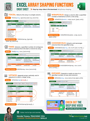
Microsoft recently released 11 new Excel functions for shaping arrays (data).
I already covered VSTACK and HSTACK which was super popular, and in this post I’m going to use some of the other new functions to do things that used to require ninja level function wrangling.
You can see the individual tutorials covered in the video or read about them at the links below.
Note: these functions are only available to Microsoft 365 users.
Download Cheat Sheet and Workbook
Enter your email address below to download the files.

Download the Excel Workbook and follow along. Note: This is a .xlsx file please ensure your browser doesn't change the file extension on download.
Watch the Video

| Function | Description |
| EXPAND | Expands or pads an array to a specified number of rows and columns. |
| TOROW | Returns the array in a single row. Useful for combining data across multiple columns and rows into a single row. |
| TOCOL | Returns the array in a single column. Useful for combining data across multiple columns and rows into a single column. |
| WRAPROWS | Lets you wrap (reshape) a row or column of values into rows, you specify the number of values in each row. |
| WRAPCOLS | Lets you wrap (reshape) a row or column of values into columns, you specify the number of values in each column. |
| DROP | Remove a specified number of contiguous rows or columns from the start or end of an array. |
| TAKE | Extract a specified number of contiguous rows or columns from the start or end of an array. |
| CHOOSEROWS | Extract rows from the specified column or columns. |
| CHOOSECOLS | Extract columns from the specified rows or rows. |
| VSTACK | Combine arrays arranged vertically (VSTACK) into a new single array. |
| HSTACK | Combine arrays arranged horizontally (HSTACK) into a new single array. |
Nested Array Shaping Functions
Individually the new array shaping functions are amazing, but team them up and you can create some super useful formulas.
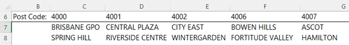
In the table below I have a list of postcodes and the corresponding suburbs:
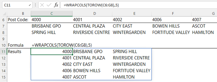
I can pivot the layout with WRAPCOLS and TOROW so that the postcodes are now in a column like so:
Or I can format it in a tabular layout with a column for the postcode and a column for the suburb with HSTACK, TOCOL and CHOOSEROWS:
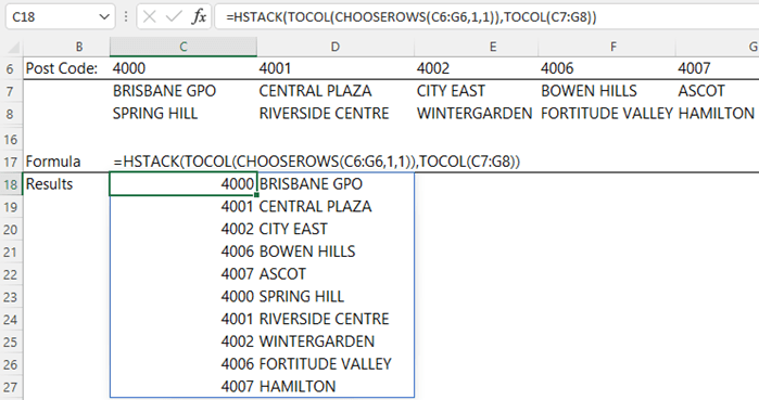
Notice how I used CHOOSEROWS to return the list of postcodes twice, hence the 1,1 in the CHOOSEROWS formula:
=HSTACK(TOCOL(CHOOSEROWS(C6:G6,1,1)),TOCOL(C7:G8))
Handling Missing Data
If there’s an uneven number of suburbs for each postcode you end up with blanks in the result:
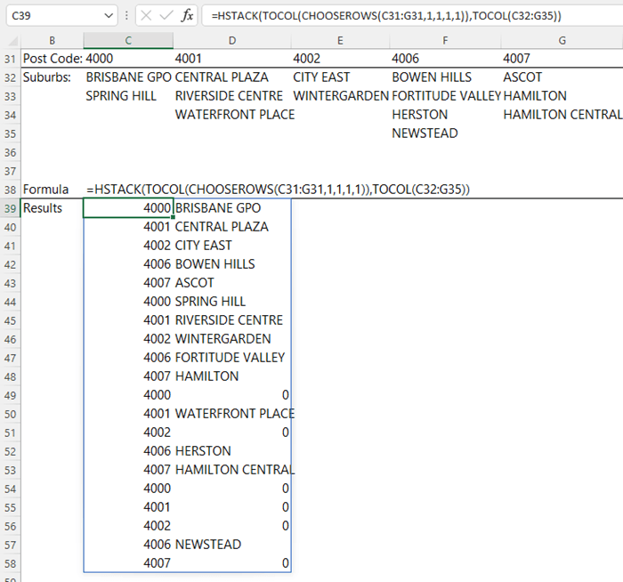
We can filter out the blanks with the FILTER function:
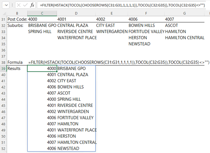
FILTER checks for blanks by repeating the second array in HSTACK returned by TOCOL:
=FILTER(HSTACK(TOCOL(CHOOSEROWS(C31:G31,1,1,1,1)),TOCOL(C32:G35)), TOCOL(C32:G35)<>"")

There might be a use for EXPAND involving a problem needing matrix math operations on two arrays on unequal size. I can’t think of a practical example, though.
Thanks for sharing, Martin. Someone did give me a use for it once, but I’ve already forgotten what it was 😀